supervision with ordinal labels
[ ]:
[1]:
#pip install pacmap KDEpy
[2]:
import numpy as np
import scanpy as sc
import pacmap
import stream2 as st2
import matplotlib.pyplot as plt
from sklearn.neighbors import NearestNeighbors
/home/jo/anaconda3/envs/stream2/lib/python3.8/site-packages/tqdm/auto.py:21: TqdmWarning: IProgress not found. Please update jupyter and ipywidgets. See https://ipywidgets.readthedocs.io/en/stable/user_install.html
  from .autonotebook import tqdm as notebook_tqdm
Load data
We directly load preprocessed data from Schiebinger 2019 subsampled to ~10% of points with geosketch
Uncomment the cell below if you wish to replicate preprocessing yourself
[3]:
adata = sc.read('../data/reprogramming/wot.h5ad')
[4]:
## download data from https://broadinstitute.github.io/wot/tutorial/
#import wot
#import pandas as pd

#PATH = '../../git/wot/notebooks/data/'
#
##---Path to input files
#FLE_COORDS_PATH ='data/fle_coords.txt'
#FULL_DS_PATH = 'data/ExprMatrix.h5ad'
#VAR_DS_PATH = 'data/ExprMatrix.var.genes.h5ad'
#CELL_DAYS_PATH = 'data/cell_days.txt'
#GENE_SETS_PATH = 'data/gene_sets.gmx'
#GENE_SET_SCORES_PATH = 'data/gene_set_scores.csv'
#CELL_SETS_PATH = 'data/cell_sets.gmt'
#MAJOR_CELL_SETS_PATH = 'data/major_cell_sets.gmt'
#SERUM_CELL_IDS_PATH = 'data/serum_cell_ids.txt'
#CELL_GROWTH_PATH = 'data/growth_gs_init.txt'
#
#coord_df = pd.read_csv(PATH+FLE_COORDS_PATH, index_col='id', sep='\t')
#days_df = pd.read_csv(PATH+CELL_DAYS_PATH, index_col='id', sep='\t')
#gene_set_df = pd.read_csv(PATH+GENE_SET_SCORES_PATH, index_col='id').rename(columns={'Trophoblast':'Trophoblast.identity'})
#cell_sets = wot.io.read_sets(PATH+CELL_SETS_PATH)
#serum_id = pd.read_csv(PATH+SERUM_CELL_IDS_PATH,header=None)
#adata = sc.read_h5ad(PATH+VAR_DS_PATH)
#
## subset labeled days
#adata.obs['label']=days_df
#adata=adata[~adata.obs['label'].isna()].copy()
#sc.pp.pca(adata)
#
## add annotations
#df=cell_sets.to_df()
#df['cell_sets'] = ''
#for c in df.columns[:-1]:
#    df.loc[df[c]>0,'cell_sets']=c
#adata.obs=adata.obs.join(df)
#adata.obs.loc[adata.obs['cell_sets'].isna(),'cell_sets']='nan'
#adata.obs['cell_sets']=adata.obs['cell_sets'].astype(str)
#
#adata.obs['cell_sets_simple']=adata.obs['cell_sets'].copy()
#adata.obs['cell_sets_simple'][adata.obs['cell_sets'].isin(['Trophoblast','SpongioTropho','ProgenitorTropho','SpiralArteryTrophoGiant'])] = 'Trophoblast'
#adata.obs['cell_sets_simple'][adata.obs['cell_sets'].isin(['Neural','RadialGlia','Neuron','Astrocyte'])] = 'Neural'
#adata.uns['cell_sets_simple_color'] = {
# 'Epithelial': '#EC8E26',
# 'IPS': '#c0c1c0',
# 'MET': '#9e50c7',
# 'Neural': '#47e026',
# 'OPC': '#7f7f7f',
# 'Stromal': '#3f4af4',
# 'Trophoblast': '#b5361a',
# 'nan': '#434342'}
#
#adata.obs['serum']='0'
#adata.obs['serum'][adata.obs.index.isin(serum_id[0].values)]='1'
#
#from geosketch import gs
#sketch_index = gs(adata.obsm['X_pca'], N=25000, replace=False,seed=0)
#s_adata = adata[sketch_index]
#s_adata.write('../data/wot.h5ad')

### compute cytotrace scores using pyrovelocity implementation
#import sys
#sys.path.append('../../pyrovelocity/pyrovelocity/')
#import cytotrace
#import sklearn
#
#PATH = '../../wot/notebooks/data/'
#FULL_DS_PATH = 'data/ExprMatrix.h5ad'
#adata_full = sc.read_h5ad(PATH+FULL_DS_PATH)
#s_adata = sc.read('../data/reprogramming/wot.h5ad')
#s_adata_full = adata_full[s_adata.obs_names].copy()
#ss_adata_full = sc.pp.subsample(s_adata_full,n_obs=5000,copy=True)
#cyto = cytotrace.cytotrace(ss_adata_full,layer=None)
#
#knnreg = sklearn.neighbors.KNeighborsRegressor(weights='distance').fit(ss_adata_full.X,cyto['CytoTRACE'])
#s_adata.obs['CytoTRACE'] = knnreg.predict(s_adata_full.X)
Supervised dimension reduction
In this dataset cells are already quite well ordered by time. Still there are discrepancies where earlier cells are sampled near the tip of the distribution, after cells from later days and vice versa
If needed we can correct the few outlier ordinal labels by voting
[5]:
k = 30

knn_label_vote = adata.obs['label'].copy()
dis, idx = NearestNeighbors(n_neighbors=k,n_jobs=30).fit(adata.obsm['X_pca']).kneighbors()

for i, x in enumerate(np.array(adata.obs['label'])[idx]):
    unique, count = np.unique(x, return_counts=1)
    argmax = np.argmax(count)
    if count[argmax] > k/2:
        knn_label_vote[i] = unique[argmax]

adata.obs['knn_label_vote'] = knn_label_vote
We perform unsupervised dimensionality reduction as baseline
[6]:
if "X_pacmap" not in adata.obsm:
    adata.obsm['X_pacmap'] = pacmap.PaCMAP(n_neighbors=k, distance='angular',random_state=0, FP_ratio=.4).fit_transform(adata.obsm['X_pca'])
sc.pl.embedding(adata,basis='X_pacmap',color=['label','cell_sets_simple','serum','CytoTRACE'],ncols=2)
/home/jo/anaconda3/envs/stream2/lib/python3.8/site-packages/scanpy/plotting/_tools/scatterplots.py:392: UserWarning: No data for colormapping provided via 'c'. Parameters 'cmap' will be ignored
  cax = scatter(
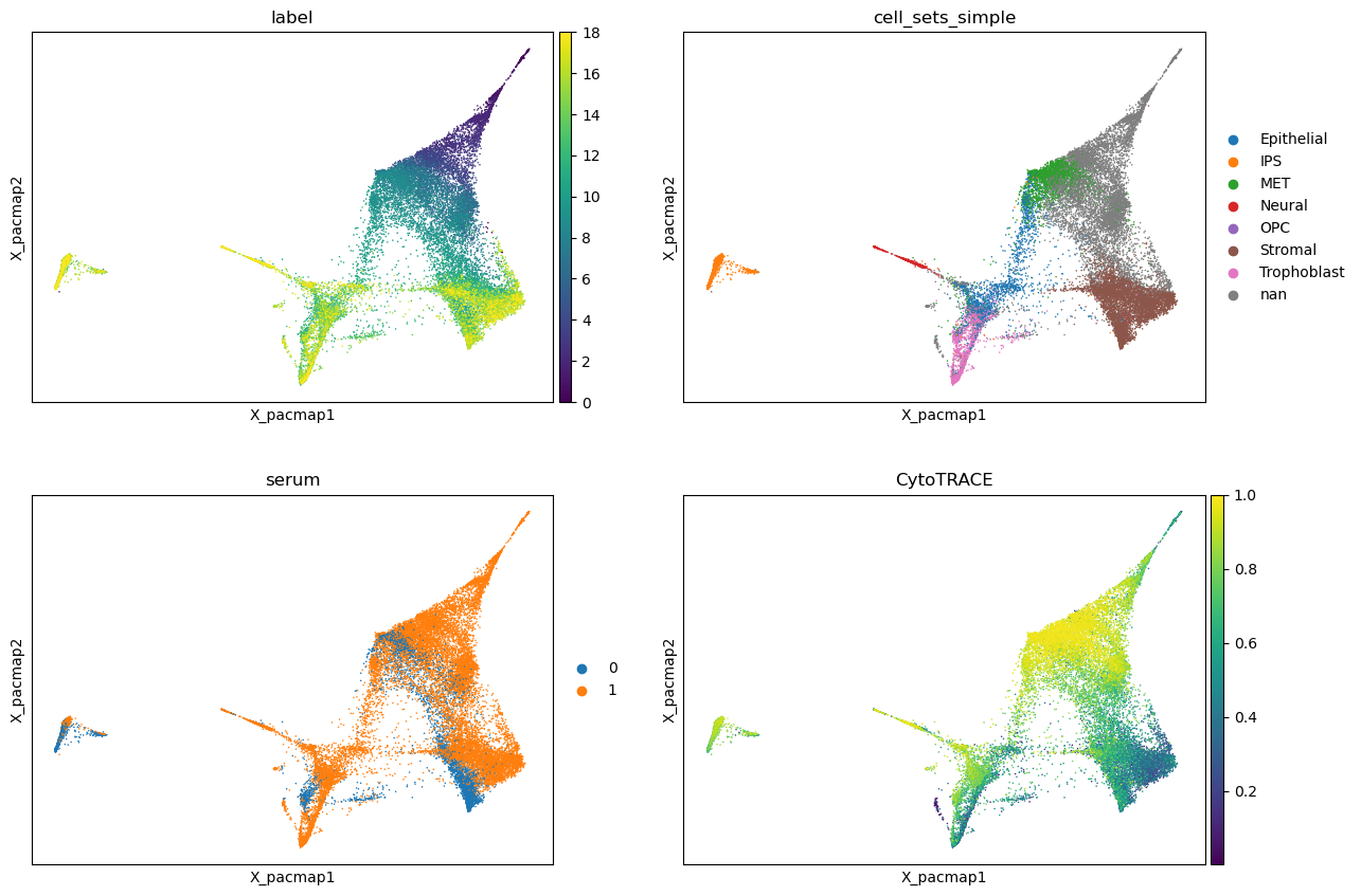
There is usually a decision to be made which notion of time we care more about respecting: pseudotime (e.g., following data density or the number of expressed genes) vs wall time. Heuristic tools such as CytoTRACE (https://cytotrace.stanford.edu/) and psupertime (https://github.com/wmacnair/psupertime) can help to define pseudotime and find a consensus with wall time labels.
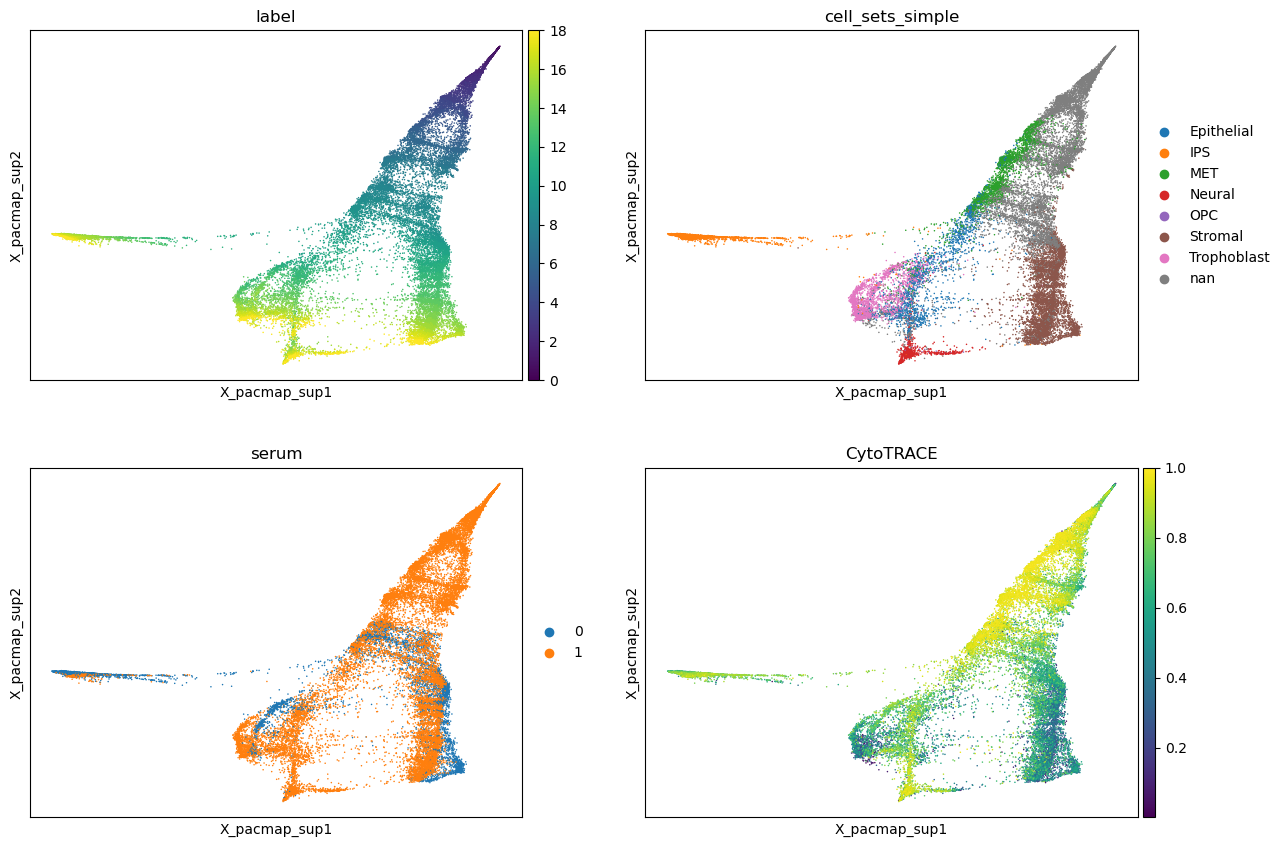
In case we decide to more closely follow wall time, a simple solution is to perform supervised dimensionality reduction by using ordinal labels and choosing a supervision strength.
[7]:
if "X_pacmap_sup" not in adata.obsm:
    knn_dists,knn_idx = st2.tl.ordinal_knn(adata,obsm='X_pca',ordinal_label='label', method='force',
                                              n_neighbors = k, n_natural = 2, metric = 'cosine')


    scaled_dist = np.ones_like(knn_idx,dtype='float32')
    pair_neighbors = pacmap.sample_neighbors_pair(adata.obsm['X_pca'], scaled_dist, knn_idx, k)
    adata.obsm['X_pacmap_sup'] = pacmap.PaCMAP(n_neighbors=k,random_state=0,FP_ratio=.4,
                                               pair_neighbors=pair_neighbors).fit_transform(adata.obsm['X_pca'])
sc.pl.embedding(adata,basis='X_pacmap_sup',color=['label','cell_sets_simple','serum','CytoTRACE'],ncols=2)
Trajectory inference
Let us seed the graph with a minimum spanning tree. We can see that 10 clusters are not enough
[8]:
adata.obsm['X_dr']=adata.obsm['X_pacmap_sup']
st2.tl.seed_graph(adata,n_clusters=10,use_weights=False)
st2.pl.graph(adata,key='seed_epg',color=['label'],show_node=1)
Seeding initial graph...
Clustering...
K-Means clustering ...
Calculating minimum spanning tree...
A simple solution is to increase the number of clusters
[9]:
st2.tl.seed_graph(adata,n_clusters=50,use_weights=False)
st2.pl.graph(adata,key='seed_epg',color=['label'],show_node=1)
Seeding initial graph...
Clustering...
K-Means clustering ...
Calculating minimum spanning tree...
The seed graph is still not ideal, e.g. for IPS cells because the start of the branch is very sparse.
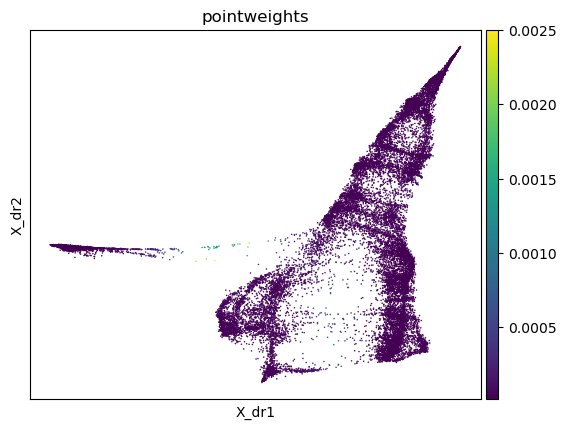
This can be improved by computing density and assigning higher weights to points in sparse regions of data
[10]:
st2.tl.get_weights(adata,bandwidth=.5,method='fft')
sc.pl.embedding(adata,basis='X_dr',color='pointweights')

st2.tl.seed_graph(adata,n_clusters=50,use_weights=True)
st2.pl.graph(adata,key='seed_epg',color=['label'],show_node=1)
Seeding initial graph...
Clustering...
K-Means clustering ...
Calculating minimum spanning tree...
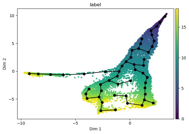
We now refine the guess by computing an unsupervised principal graph
We can make use of GPU acceleration with the cupy library; if you don’t have one set GPU=False
[11]:
st2.tl.learn_graph(adata,n_nodes=100,epg_alpha=0.02,epg_mu=0.1,epg_lambda=0.01,
                   use_weights=True, GPU=False, store_evolution=True,
                   #max_candidates={'AddNode2Node': 15, 'BisectEdge': 10, 'ShrinkEdge':10},
                   verbose=1,)
st2.pl.graph(adata,key='epg',color=['label','cell_sets_simple'],alpha=.2,size=2)
Constructing tree 1 of 1 / Subset 1 of 1
Computing EPG with  100  nodes on  25000  points and  2  dimensions

BARCODE ENERGY  NNODES  NEDGES  NRIBS   NSTARS  NRAYS   NRAYS2  MSE     MSEP    FVE     FVEP    UE      UR      URN     URN2    URSD

7||51   0.5845  51      50      35      7       0       0       0.2413  0.1981  0.9929  0.9942  0.3223  0.0209  1.0646  54.2967 0
6||52   0.5588  52      51      38      6       0       0       0.2399  0.2001  0.9929  0.9941  0.3064  0.0125  0.6525  33.9303 0
5||53   0.5745  53      52      41      5       0       0       0.2497  0.2118  0.9926  0.9938  0.295   0.0298  1.578   83.6334 0
5||54   0.5526  54      53      42      5       0       0       0.2425  0.2077  0.9929  0.9939  0.2835  0.0266  1.4389  77.7016 0
5||55   0.5486  55      54      43      5       0       0       0.2458  0.212   0.9928  0.9938  0.2731  0.0297  1.6312  89.7157 0
5||56   0.5396  56      55      44      5       0       0       0.25    0.2178  0.9926  0.9936  0.2593  0.0303  1.6951  94.9246 0
4||57   0.5259  57      56      47      4       0       0       0.2494  0.2188  0.9927  0.9936  0.2493  0.0273  1.5565  88.7177 0
4||58   0.5159  58      57      48      4       0       0       0.2456  0.2167  0.9928  0.9936  0.2446  0.0258  1.4959  86.7612 0
4||59   0.5059  59      58      49      4       0       0       0.2364  0.2067  0.993   0.9939  0.2445  0.025   1.4779  87.1947 0
4||60   0.504   60      59      50      4       0       0       0.233   0.2042  0.9931  0.994   0.2456  0.0254  1.5242  91.4533 0
3||61   0.4946  61      60      53      3       0       0       0.2281  0.2002  0.9933  0.9941  0.2437  0.0228  1.3935  85.0025 0
3||62   0.4906  62      61      54      3       0       0       0.2282  0.2004  0.9933  0.9941  0.2408  0.0216  1.342   83.2028 0
3||63   0.4836  63      62      55      3       0       0       0.2274  0.2009  0.9933  0.9941  0.2361  0.0201  1.2674  79.8435 0
3||64   0.4784  64      63      56      3       0       0       0.2251  0.2001  0.9934  0.9941  0.2332  0.0201  1.2884  82.4596 0
3||65   0.4695  65      64      57      3       0       0       0.2189  0.1951  0.9936  0.9943  0.2303  0.0202  1.3161  85.5468 0
3||66   0.4647  66      65      58      3       0       0       0.2178  0.1951  0.9936  0.9943  0.2254  0.0215  1.4165  93.4906 0
3||67   0.4592  67      66      59      3       0       0       0.2157  0.1932  0.9936  0.9943  0.2226  0.0209  1.3994  93.762  0
3||68   0.4559  68      67      60      3       0       0       0.2141  0.1918  0.9937  0.9944  0.2213  0.0205  1.3927  94.7014 0
3||69   0.4501  69      68      61      3       0       0       0.2119  0.19    0.9938  0.9944  0.2192  0.019   1.3121  90.5346 0
3||70   0.4451  70      69      62      3       0       0       0.2096  0.1884  0.9938  0.9945  0.2163  0.0192  1.3435  94.0419 0
3||71   0.442   71      70      63      3       0       0       0.208   0.1867  0.9939  0.9945  0.2142  0.0197  1.4021  99.5515 0
3||72   0.4355  72      71      64      3       0       0       0.203   0.1828  0.994   0.9946  0.214   0.0185  1.3288  95.6731 0
3||73   0.4339  73      72      65      3       0       0       0.2035  0.1831  0.994   0.9946  0.2103  0.0201  1.4665  107.0509        0
3||74   0.4279  74      73      66      3       0       0       0.1996  0.18    0.9941  0.9947  0.209   0.0193  1.4271  105.6087        0
3||75   0.4242  75      74      67      3       0       0       0.1987  0.1793  0.9941  0.9947  0.2067  0.0188  1.4063  105.4736        0
3||76   0.4182  76      75      68      3       0       0       0.1941  0.175   0.9943  0.9948  0.2054  0.0187  1.4208  107.9839        0
3||77   0.413   77      76      69      3       0       0       0.1894  0.171   0.9944  0.995   0.2041  0.0195  1.4993  115.4427        0
3||78   0.4113  78      77      70      3       0       0       0.1902  0.1721  0.9944  0.9949  0.2015  0.0196  1.5296  119.307 0
3||79   0.4081  79      78      71      3       0       0       0.1896  0.1717  0.9944  0.9949  0.1991  0.0194  1.5312  120.9646        0
3||80   0.404   80      79      72      3       0       0       0.1874  0.1703  0.9945  0.995   0.197   0.0196  1.5717  125.7345        0
3||81   0.4011  81      80      73      3       0       0       0.1871  0.1707  0.9945  0.995   0.1947  0.0193  1.5664  126.8775        0
3||82   0.3964  82      81      74      3       0       0       0.184   0.1675  0.9946  0.9951  0.1942  0.0182  1.4938  122.492 0
3||83   0.3925  83      82      75      3       0       0       0.1816  0.1659  0.9947  0.9951  0.1919  0.019   1.5747  130.7019        0
3||84   0.3875  84      83      76      3       0       0       0.1765  0.1614  0.9948  0.9952  0.1917  0.0194  1.6265  136.6294        0
3||85   0.3866  85      84      77      3       0       0       0.1786  0.1629  0.9947  0.9952  0.1898  0.0182  1.5454  131.3622        0
3||86   0.3817  86      85      78      3       0       0       0.1744  0.1593  0.9949  0.9953  0.1882  0.0191  1.64    141.0405        0
3||87   0.3807  87      86      79      3       0       0       0.176   0.1608  0.9948  0.9953  0.1866  0.0181  1.5748  137.0036        0
3||88   0.3775  88      87      80      3       0       0       0.1746  0.1599  0.9949  0.9953  0.1845  0.0184  1.6178  142.3653        0
3||89   0.3744  89      88      81      3       0       0       0.1728  0.1585  0.9949  0.9953  0.1832  0.0184  1.6407  146.0203        0
3||90   0.3687  90      89      82      3       0       0       0.1664  0.1525  0.9951  0.9955  0.1838  0.0185  1.6659  149.9304        0
3||91   0.366   91      90      83      3       0       0       0.1665  0.1531  0.9951  0.9955  0.1813  0.0182  1.6587  150.9389        0
3||92   0.3652  92      91      84      3       0       0       0.1677  0.1545  0.9951  0.9955  0.1794  0.0181  1.6624  152.9364        0
3||93   0.3626  93      92      85      3       0       0       0.1682  0.1551  0.995   0.9954  0.1769  0.0175  1.6253  151.1492        0
3||94   0.3597  94      93      86      3       0       0       0.1667  0.1539  0.9951  0.9955  0.1756  0.0174  1.634   153.5971        0
3||95   0.3563  95      94      87      3       0       0       0.1644  0.1515  0.9952  0.9955  0.1741  0.0178  1.692   160.7378        0
3||96   0.3518  96      95      88      3       0       0       0.1609  0.1484  0.9953  0.9956  0.1731  0.0177  1.7028  163.4646        0
3||97   0.3509  97      96      89      3       0       0       0.1607  0.1484  0.9953  0.9956  0.172   0.0182  1.7628  170.9886        0
3||98   0.3486  98      97      90      3       0       0       0.1612  0.1494  0.9953  0.9956  0.1698  0.0175  1.7184  168.4026        0
3||99   0.3453  99      98      91      3       0       0       0.1581  0.1464  0.9953  0.9957  0.1691  0.0181  1.7913  177.3353        0
3||100  0.3437  100     99      92      3       0       0       0.1584  0.1467  0.9953  0.9957  0.1679  0.0174  1.7444  174.4388        0
504.8498  seconds elapsed
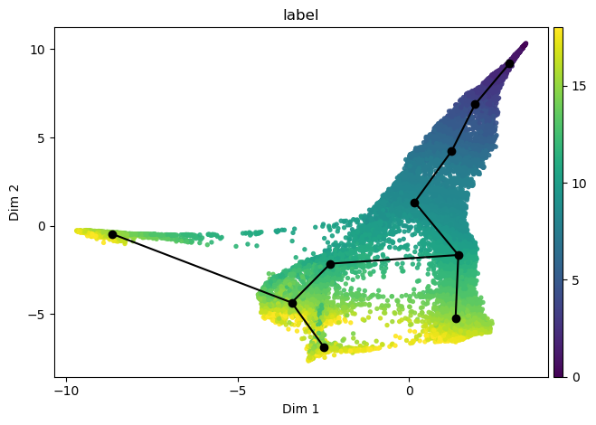
Since we used store_evolution=True we have access to graphs for any number of nodes between n_clusters of the seed graph and n_nodes
[12]:
st2.tl.use_graph_with_n_nodes(adata,n_nodes=80)
st2.pl.graph(adata,key='epg',color=['label'])
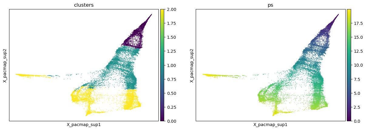
While the structure is better than the seed graph, the result is suboptimal and some branches do not follow ordinal labels. We can compute a supervised principal graph to get better results Ordinal labels should be smoothed into a continuous variable before learning the supervised graph (here they are already densely sampled so we won’t need this - we just discretize them into 3 bins as an example)
[12]:
#define a root point
root_idx = 0
time = adata.obs['label']
bins = np.histogram(time, bins=3)[1]
adata.obs['clusters'] = np.digitize(time, bins[1:], right=True)

st2.tl.smooth_ordinal_labels(adata, root_idx, ordinal_label='clusters', obsm="X_pacmap_sup")
sc.pl.embedding(adata,'X_pacmap_sup',color=['clusters','ps'])
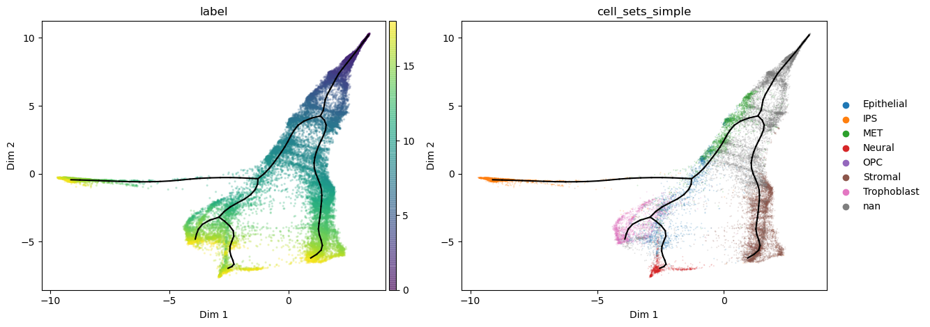
We then need to define 3 extra variables: root cell, ordinal labels to follow and supervision strength - ordinal_supervision_strength = 1 means equal importance to respecting ordinal labels vs natural data order, - ordinal_supervision_strength = 10 means following ordinal labels is 10 times more important
[13]:
adata2=adata.copy()
st2.tl.learn_graph(
    adata2,
    n_nodes=100,epg_alpha=0.02,epg_mu=0.1,epg_lambda=0.01,
    GPU=False,store_evolution=True,use_weights=True,use_seed=True,
    max_candidates={'AddNode2Node': 15, 'BisectEdge': 10, 'ShrinkEdge':10},verbose=1,

    # supervision parameters
    ordinal_label = 'knn_label_vote',                            #define the ordinal vector to follow
    ordinal_root_point = root_idx,                               #define a root point (e.g., cell with lowest ordinal value)
    ordinal_supervision_strength = 1,                            #define strength of supervision in [0, +inf).
)

st2.pl.graph(adata2,key='epg',color=['label','cell_sets_simple'],alpha=.2,size=2)
#st2.pl.graph(adata2,key='epg',color=['label','cell_sets_simple'],alpha=.2,size=2,
#            fig_path=f'figures/reprogramming/shareseq_stream_umap.png',save_fig=True)
Constructing tree 1 of 1 / Subset 1 of 1
The elastic matrix is being used. Edge configuration will be ignored
Computing EPG with  100  nodes on  25000  points and  2  dimensions

BARCODE ENERGY  NNODES  NEDGES  NRIBS   NSTARS  NRAYS   NRAYS2  MSE     MSEP    FVE     FVEP    UE      UR      URN     URN2    URSD

6||52   0.5399  52      51      38      6       0       0       0.2372  0.1969  0.993   0.9942  0.2922  0.0105  0.5463  28.4089 0
6||53   0.5101  53      52      39      6       0       0       0.2192  0.1814  0.9935  0.9947  0.2812  0.0097  0.5153  27.3126 0
5||54   0.4987  54      53      42      5       0       0       0.2145  0.1766  0.9937  0.9948  0.2735  0.0107  0.5777  31.1957 0
5||55   0.4846  55      54      43      5       0       0       0.2083  0.1728  0.9939  0.9949  0.2663  0.01    0.5492  30.2048 0
5||56   0.4768  56      55      44      5       0       0       0.2086  0.1752  0.9939  0.9948  0.2578  0.0105  0.5854  32.7803 0
4||57   0.4747  57      56      47      4       0       0       0.2199  0.1873  0.9935  0.9945  0.2465  0.0082  0.4667  26.5997 0
4||58   0.4691  58      57      48      4       0       0       0.2143  0.1813  0.9937  0.9947  0.2474  0.0075  0.4364  25.3112 0
4||59   0.4658  59      58      49      4       0       0       0.2121  0.1794  0.9938  0.9947  0.246   0.0078  0.4583  27.0391 0
4||60   0.4576  60      59      50      4       0       0       0.214   0.1825  0.9937  0.9946  0.236   0.0076  0.4558  27.3464 0
4||61   0.446   61      60      51      4       0       0       0.2086  0.1793  0.9939  0.9947  0.2298  0.0075  0.4593  28.0157 0
3||62   0.4378  62      61      54      3       0       0       0.2094  0.182   0.9938  0.9946  0.2203  0.008   0.4959  30.7479 0
3||63   0.4314  63      62      55      3       0       0       0.2099  0.1845  0.9938  0.9946  0.2136  0.0079  0.5     31.4999 0
3||64   0.4273  64      63      56      3       0       0       0.2075  0.183   0.9939  0.9946  0.2115  0.0083  0.5293  33.8736 0
3||65   0.4213  65      64      57      3       0       0       0.2066  0.1828  0.9939  0.9946  0.2068  0.0079  0.5109  33.2085 0
3||66   0.4193  66      65      58      3       0       0       0.2036  0.1797  0.994   0.9947  0.2075  0.0082  0.5399  35.6353 0
3||67   0.4132  67      66      59      3       0       0       0.2002  0.1775  0.9941  0.9948  0.205   0.008   0.5379  36.0367 0
3||68   0.4129  68      67      60      3       0       0       0.1989  0.1762  0.9941  0.9948  0.2062  0.0078  0.5316  36.1516 0
3||69   0.4078  69      68      61      3       0       0       0.1977  0.176   0.9942  0.9948  0.2025  0.0076  0.5267  36.344  0
3||70   0.4049  70      69      62      3       0       0       0.1959  0.1745  0.9942  0.9949  0.2013  0.0076  0.5335  37.3476 0
3||71   0.4029  71      70      63      3       0       0       0.1953  0.174   0.9942  0.9949  0.2002  0.0075  0.5302  37.6442 0
3||72   0.3977  72      71      64      3       0       0       0.1926  0.1718  0.9943  0.9949  0.1979  0.0072  0.5198  37.4246 0
3||73   0.3939  73      72      65      3       0       0       0.1915  0.1712  0.9944  0.995   0.1952  0.0073  0.5296  38.6616 0
3||74   0.3909  74      73      66      3       0       0       0.1911  0.1712  0.9944  0.995   0.1927  0.0072  0.5305  39.255  0
3||75   0.3856  75      74      67      3       0       0       0.1908  0.1719  0.9944  0.9949  0.1877  0.0071  0.535   40.1281 0
3||76   0.3834  76      75      68      3       0       0       0.1889  0.1703  0.9944  0.995   0.1871  0.0074  0.5648  42.9214 0
3||77   0.3804  77      76      69      3       0       0       0.1882  0.1702  0.9945  0.995   0.1845  0.0077  0.5937  45.7116 0
3||78   0.379   78      77      70      3       0       0       0.1872  0.1694  0.9945  0.995   0.1837  0.0081  0.6323  49.317  0
3||79   0.3758  79      78      71      3       0       0       0.1863  0.1692  0.9945  0.995   0.182   0.0075  0.5893  46.5518 0
3||80   0.373   80      79      72      3       0       0       0.1838  0.1669  0.9946  0.9951  0.1814  0.0078  0.6238  49.9013 0
3||81   0.3714  81      80      73      3       0       0       0.1854  0.1688  0.9945  0.995   0.1785  0.0076  0.6147  49.7869 0
3||82   0.3676  82      81      74      3       0       0       0.1828  0.167   0.9946  0.9951  0.1773  0.0075  0.6111  50.1088 0
3||83   0.3659  83      82      75      3       0       0       0.1807  0.1648  0.9947  0.9951  0.1782  0.007   0.5834  48.4181 0
3||84   0.3636  84      83      76      3       0       0       0.1789  0.1637  0.9947  0.9952  0.1775  0.0071  0.6004  50.4372 0
3||85   0.3615  85      84      77      3       0       0       0.1745  0.1589  0.9949  0.9953  0.1797  0.0073  0.6225  52.9125 0
3||86   0.3559  86      85      78      3       0       0       0.1709  0.1557  0.995   0.9954  0.1769  0.0082  0.7028  60.4418 0
3||87   0.35    87      86      79      3       0       0       0.1667  0.1518  0.9951  0.9955  0.175   0.0084  0.7336  63.8214 0
3||88   0.352   88      87      80      3       0       0       0.1659  0.1512  0.9951  0.9955  0.1764  0.0097  0.8505  74.8418 0
3||89   0.3494  89      88      81      3       0       0       0.1649  0.1502  0.9951  0.9956  0.1747  0.0098  0.8724  77.6478 0
3||90   0.3446  90      89      82      3       0       0       0.1625  0.1483  0.9952  0.9956  0.1726  0.0095  0.8573  77.1608 0
3||91   0.338   91      90      83      3       0       0       0.1578  0.144   0.9954  0.9958  0.1721  0.0081  0.734   66.7928 0
3||92   0.3358  92      91      84      3       0       0       0.1584  0.1449  0.9953  0.9957  0.1696  0.0078  0.7171  65.9768 0
3||93   0.333   93      92      85      3       0       0       0.154   0.1404  0.9955  0.9959  0.1711  0.0079  0.7343  68.2859 0
3||94   0.3319  94      93      86      3       0       0       0.1532  0.1398  0.9955  0.9959  0.171   0.0077  0.7223  67.8992 0
3||95   0.3289  95      94      87      3       0       0       0.151   0.1379  0.9956  0.9959  0.1704  0.0075  0.7119  67.6336 0
3||96   0.3249  96      95      88      3       0       0       0.1503  0.1375  0.9956  0.996   0.167   0.0076  0.7295  70.0339 0
3||97   0.3208  97      96      89      3       0       0       0.1484  0.1361  0.9956  0.996   0.1647  0.0076  0.7391  71.6936 0
3||98   0.3178  98      97      90      3       0       0       0.1463  0.1342  0.9957  0.996   0.1638  0.0077  0.7564  74.1267 0
3||99   0.3168  99      98      91      3       0       0       0.1456  0.1335  0.9957  0.9961  0.1634  0.0078  0.773   76.5269 0
3||100  0.3145  100     99      92      3       0       0       0.1445  0.1327  0.9957  0.9961  0.1622  0.0078  0.783   78.2977 0
649.5394  seconds elapsed
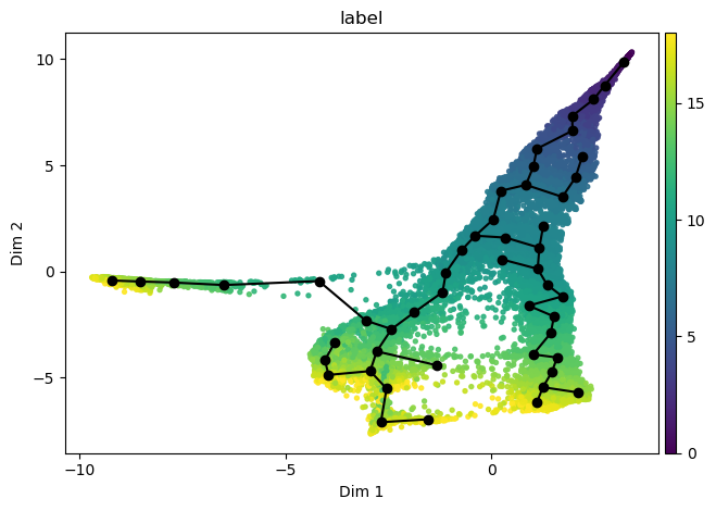
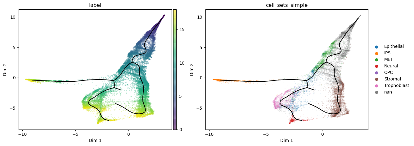
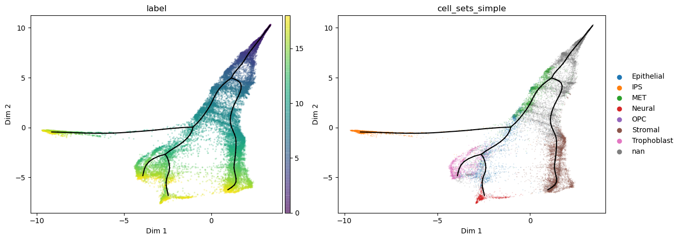
For best results we infer the graph without the max candidates heuristic and fine tune nodes and supervision strength parameters
[14]:
adata2=adata.copy()
st2.tl.learn_graph(
    adata2,
    n_nodes=110,epg_alpha=0.02,epg_mu=0.1,epg_lambda=0.01,
    GPU=False,store_evolution=True,use_weights=True,use_seed=True,verbose=1,

    # supervision parameters
    ordinal_label = 'knn_label_vote',                            #define the ordinal vector to follow
    ordinal_root_point = root_idx,                               #define a root point (e.g., cell with lowest ordinal value)
    ordinal_supervision_strength = 2.5,                            #define strength of supervision in [0, +inf).
)

st2.pl.graph(adata2,key='epg',color=['label','cell_sets_simple'],alpha=.2,size=2)
#st2.pl.graph(adata2,key='epg',color=['label','cell_sets_simple'],alpha=.2,size=2,
#            fig_path=f'figures/reprogramming/shareseq_stream_umap.png',save_fig=True)
Constructing tree 1 of 1 / Subset 1 of 1
The elastic matrix is being used. Edge configuration will be ignored
Computing EPG with  110  nodes on  25000  points and  2  dimensions

BARCODE ENERGY  NNODES  NEDGES  NRIBS   NSTARS  NRAYS   NRAYS2  MSE     MSEP    FVE     FVEP    UE      UR      URN     URN2    URSD

6||52   0.5412  52      51      38      6       0       0       0.2401  0.199   0.9929  0.9941  0.2913  0.0098  0.5105  26.5441 0
6||53   0.519   53      52      39      6       0       0       0.223   0.1834  0.9934  0.9946  0.2858  0.0102  0.538   28.5148 0
5||54   0.497   54      53      42      5       0       0       0.2158  0.1771  0.9936  0.9948  0.271   0.0102  0.5486  29.6251 0
5||55   0.4798  55      54      43      5       0       0       0.2043  0.1674  0.994   0.9951  0.2663  0.0091  0.5032  27.6746 0
5||56   0.4665  56      55      44      5       0       0       0.1998  0.1666  0.9941  0.9951  0.2571  0.0096  0.5382  30.1379 0
4||57   0.4697  57      56      47      4       0       0       0.215   0.1813  0.9937  0.9947  0.2481  0.0066  0.3762  21.4451 0
4||58   0.4649  58      57      48      4       0       0       0.2112  0.1781  0.9938  0.9948  0.247   0.0066  0.3853  22.3459 0
4||59   0.4512  59      58      49      4       0       0       0.2119  0.1816  0.9938  0.9947  0.2328  0.0065  0.3856  22.7532 0
3||60   0.4411  60      59      52      3       0       0       0.2133  0.1849  0.9937  0.9946  0.2208  0.0069  0.4167  25.0011 0
3||61   0.4379  61      60      53      3       0       0       0.2097  0.1824  0.9938  0.9946  0.2212  0.007   0.4263  26.0067 0
3||62   0.4335  62      61      54      3       0       0       0.2082  0.1813  0.9939  0.9947  0.2186  0.0068  0.4224  26.1884 0
3||63   0.4281  63      62      55      3       0       0       0.2062  0.1802  0.9939  0.9947  0.2153  0.0065  0.4118  25.9435 0
3||64   0.425   64      63      56      3       0       0       0.2047  0.1786  0.994   0.9947  0.2142  0.0061  0.3881  24.8405 0
3||65   0.4185  65      64      57      3       0       0       0.2044  0.1798  0.994   0.9947  0.2078  0.0062  0.4006  26.0378 0
3||66   0.4161  66      65      58      3       0       0       0.2015  0.1775  0.9941  0.9948  0.2086  0.006   0.396   26.1382 0
3||67   0.4135  67      66      59      3       0       0       0.2007  0.1771  0.9941  0.9948  0.2066  0.0062  0.4129  27.6627 0
3||68   0.4115  68      67      60      3       0       0       0.199   0.1763  0.9941  0.9948  0.206   0.0065  0.4402  29.9334 0
3||69   0.4085  69      68      61      3       0       0       0.1962  0.1739  0.9942  0.9949  0.2063  0.0059  0.4103  28.3074 0
3||70   0.4054  70      69      62      3       0       0       0.1941  0.1721  0.9943  0.9949  0.2054  0.0059  0.4147  29.0308 0
3||71   0.4002  71      70      63      3       0       0       0.1945  0.1732  0.9943  0.9949  0.1995  0.0063  0.4446  31.5657 0
3||72   0.3967  72      71      64      3       0       0       0.1932  0.1725  0.9943  0.9949  0.1975  0.0061  0.441   31.7502 0
3||73   0.3942  73      72      65      3       0       0       0.192   0.1715  0.9943  0.995   0.1963  0.0059  0.432   31.5345 0
3||74   0.3878  74      73      66      3       0       0       0.192   0.1723  0.9943  0.9949  0.1898  0.006   0.4439  32.8482 0
3||75   0.3856  75      74      67      3       0       0       0.1909  0.1719  0.9944  0.9949  0.1888  0.0059  0.4424  33.1787 0
3||76   0.3828  76      75      68      3       0       0       0.1904  0.1716  0.9944  0.9949  0.1869  0.0056  0.4235  32.1886 0
3||77   0.3812  77      76      69      3       0       0       0.189   0.1706  0.9944  0.995   0.1867  0.0056  0.4288  33.0208 0
3||78   0.3755  78      77      70      3       0       0       0.1913  0.1742  0.9944  0.9949  0.1785  0.0057  0.4429  34.5424 0
3||79   0.3715  79      78      71      3       0       0       0.1896  0.1734  0.9944  0.9949  0.1764  0.0055  0.4356  34.4134 0
3||80   0.3707  80      79      72      3       0       0       0.188   0.1717  0.9945  0.9949  0.1773  0.0054  0.4305  34.4403 0
3||81   0.3695  81      80      73      3       0       0       0.1853  0.1694  0.9945  0.995   0.1787  0.0054  0.4414  35.7557 0
3||82   0.3684  82      81      74      3       0       0       0.1832  0.1675  0.9946  0.9951  0.1799  0.0052  0.429   35.1775 0
3||83   0.3629  83      82      75      3       0       0       0.1845  0.1692  0.9946  0.995   0.1734  0.005   0.414   34.3588 0
3||84   0.3602  84      83      76      3       0       0       0.1828  0.1676  0.9946  0.9951  0.1725  0.0048  0.4054  34.0569 0
3||85   0.3584  85      84      77      3       0       0       0.1814  0.1664  0.9947  0.9951  0.1721  0.0049  0.42    35.6965 0
3||86   0.3573  86      85      78      3       0       0       0.1809  0.1659  0.9947  0.9951  0.1716  0.0049  0.4198  36.1012 0
3||87   0.3538  87      86      79      3       0       0       0.1815  0.1671  0.9947  0.9951  0.1675  0.0048  0.4205  36.5866 0
3||88   0.3521  88      87      80      3       0       0       0.1802  0.1659  0.9947  0.9951  0.1672  0.0046  0.4049  35.634  0
3||89   0.3505  89      88      81      3       0       0       0.181   0.1672  0.9947  0.9951  0.1646  0.0049  0.4398  39.1449 0
3||90   0.3462  90      89      82      3       0       0       0.1797  0.1662  0.9947  0.9951  0.1616  0.0049  0.4365  39.2885 0
3||91   0.3445  91      90      83      3       0       0       0.178   0.1645  0.9948  0.9952  0.1617  0.0048  0.4362  39.6951 0
3||92   0.3428  92      91      84      3       0       0       0.1792  0.1663  0.9947  0.9951  0.1588  0.0047  0.4367  40.1778 0
3||93   0.3398  93      92      85      3       0       0       0.1771  0.1648  0.9948  0.9951  0.1581  0.0046  0.4281  39.8142 0
3||94   0.3403  94      93      86      3       0       0       0.1765  0.1645  0.9948  0.9952  0.1578  0.006   0.5667  53.2701 0
3||95   0.3382  95      94      87      3       0       0       0.1756  0.1637  0.9948  0.9952  0.1565  0.0061  0.5751  54.6366 0
3||96   0.337   96      95      88      3       0       0       0.175   0.1632  0.9948  0.9952  0.156   0.006   0.5772  55.4137 0
3||97   0.3352  97      96      89      3       0       0       0.1738  0.1618  0.9949  0.9952  0.1558  0.0056  0.5465  53.013  0
3||98   0.3346  98      97      90      3       0       0       0.1699  0.1579  0.995   0.9953  0.1584  0.0063  0.6125  60.0286 0
3||99   0.3276  99      98      91      3       0       0       0.1609  0.1489  0.9953  0.9956  0.1619  0.0048  0.4729  46.8199 0
3||100  0.3248  100     99      92      3       0       0       0.1546  0.1423  0.9954  0.9958  0.1655  0.0046  0.4598  45.9756 0
3||101  0.3179  101     100     93      3       0       0       0.1512  0.1396  0.9955  0.9959  0.1619  0.0047  0.4787  48.35   0
3||102  0.3111  102     101     94      3       0       0       0.1446  0.1328  0.9957  0.9961  0.1619  0.0047  0.4748  48.4303 0
3||103  0.3094  103     102     95      3       0       0       0.1459  0.1344  0.9957  0.996   0.1588  0.0047  0.4801  49.4511 0
3||104  0.3052  104     103     96      3       0       0       0.1431  0.1319  0.9958  0.9961  0.1573  0.0048  0.4973  51.7183 0
3||105  0.3013  105     104     97      3       0       0       0.138   0.1265  0.9959  0.9963  0.1592  0.0041  0.4306  45.2159 0
3||106  0.3005  106     105     98      3       0       0       0.1352  0.1238  0.996   0.9964  0.1597  0.0056  0.5914  62.6914 0
3||107  0.2992  107     106     99      3       0       0       0.136   0.1248  0.996   0.9963  0.158   0.0052  0.5604  59.9578 0
3||108  0.296   108     107     100     3       0       0       0.1333  0.1224  0.9961  0.9964  0.1575  0.0053  0.5733  61.9193 0
3||109  0.2947  109     108     101     3       0       0       0.1318  0.121   0.9961  0.9964  0.1577  0.0053  0.5813  63.3669 0
3||110  0.2904  110     109     102     3       0       0       0.1299  0.1192  0.9962  0.9965  0.1566  0.004   0.4389  48.281  0
1431.2766  seconds elapsed
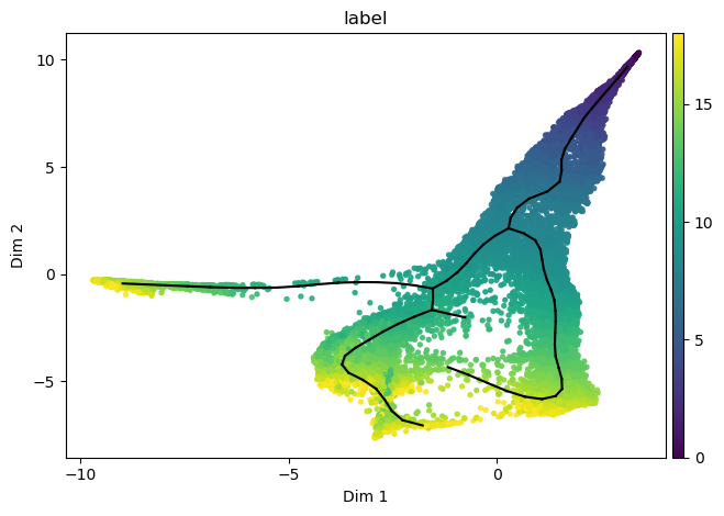
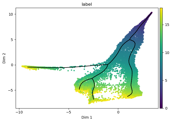
[15]:
st2.tl.use_graph_with_n_nodes(adata2,n_nodes=110)
st2.pl.graph(adata2,key='epg',color=['label'])
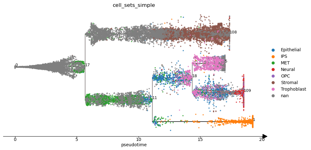
Pseudotime and trajectory plots
[25]:
st2.tl.infer_pseudotime(adata2,0)
#jitter to prevent bug for equal pseudotime values
adata2.obs['label_plot']=adata2.obs['label']+1e-20*np.random.random(len(adata2))
st2.pl.stream_sc(adata2,source=0,preference=[],dist_scale=.5,color=['cell_sets_simple'],fig_size=(10,5))
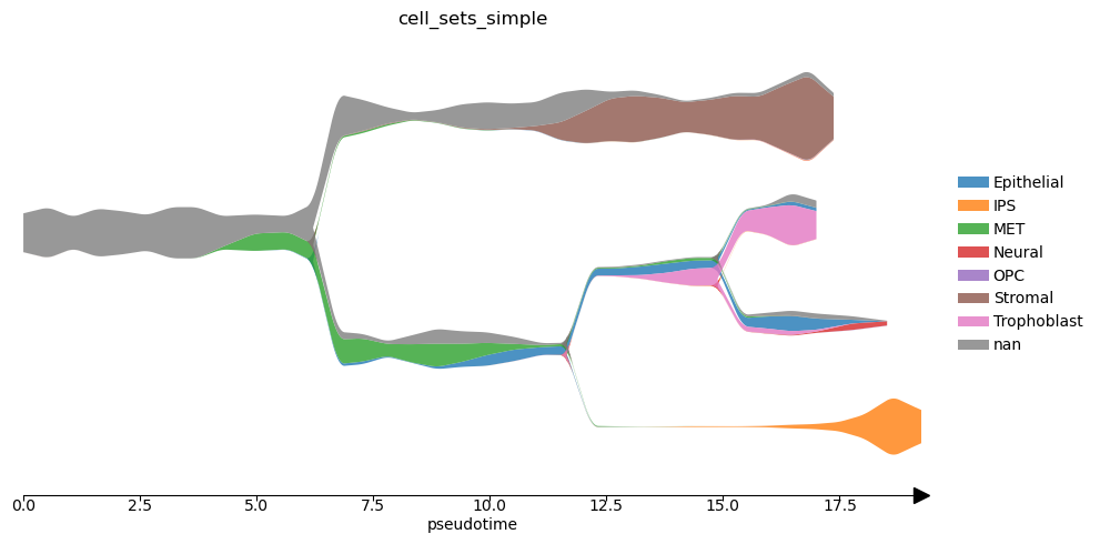
#show
st2.pl.stream(adata2,source=0,preference=[],factor_min_win=2.5,color=['cell_sets_simple'],fig_size=(10,5),
fig_path=f'figures/reprogramming/shareseq_stream_cell_sets_simple',)
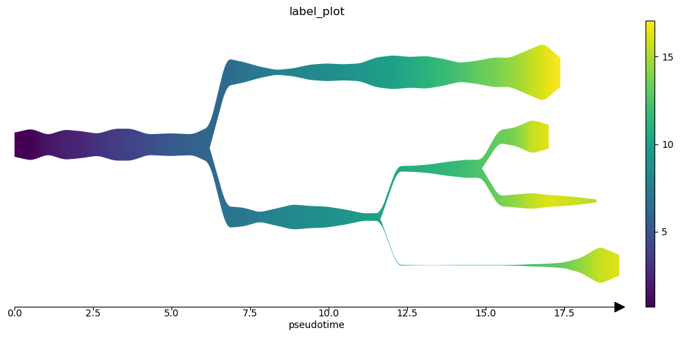
st2.pl.stream(adata2,source=0,preference=[],factor_min_win=2.5,color=['label_plot'],fig_size=(10,5),
fig_path=f'figures/reprogramming/shareseq_stream_timepoints',)
#save png
st2.pl.stream(adata2,source=0,preference=[],factor_min_win=2.5,color=['cell_sets_simple'],fig_size=(10,5),
fig_path=f'figures/reprogramming/shareseq_stream_cell_sets_simple',save_fig=True,fig_format='png')
st2.pl.stream(adata2,source=0,preference=[],factor_min_win=2.5,color=['label_plot'],fig_size=(10,5),
fig_path=f'figures/reprogramming/shareseq_stream_timepoints',save_fig=True,fig_format='png')
#save pdf
st2.pl.stream(adata2,source=0,preference=[],factor_min_win=2.5,color=['cell_sets_simple'],fig_size=(10,5),
fig_path=f'figures/reprogramming/shareseq_stream_cell_sets_simple',save_fig=True,fig_format='pdf')
st2.pl.stream(adata2,source=0,preference=[],factor_min_win=2.5,color=['label_plot'],fig_size=(10,5),
fig_path=f'figures/reprogramming/shareseq_stream_timepoints',save_fig=True,fig_format='pdf')
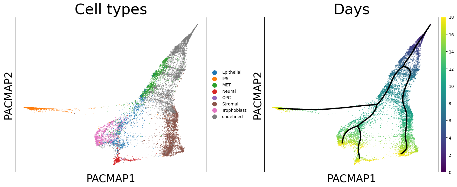
[33]:
f,axs=plt.subplots(1,2,figsize=(15,6))

adata2.obs['cell_sets_simple_plot'] = adata2.obs['cell_sets_simple'].replace('nan','undefined')
annot=['cell_sets_simple_plot','label',]
annot_name=['Cell types','Days',]

nodep=adata2.uns['epg']['node_pos']
edges=adata2.uns['epg']['edge']

adata2.obsm['X_umap']=adata2.obsm['X_pacmap_sup']
for i,key in enumerate(annot):
    ax=axs[i]
    if i==1:
        ax=sc.pl.umap(adata2,color=key,cmap='viridis',ax=ax,show=False)
        for e in edges:
            ax.plot(*nodep[e].T,linewidth=3,color='k')
    else:
        ax=sc.pl.umap(adata2,color=key,ax=ax,show=False)

    ax.set_title(annot_name[i],fontsize=35)
    ax.set_xlabel('PACMAP1',fontsize=25)
    ax.set_ylabel('PACMAP2',fontsize=25)
    if i!=1:
        #ax.legend(prop=dict(size=18),bbox_to_anchor=[1.2, 0.5], loc='center')
        for lh in ax.get_legend().legendHandles:
            lh._sizes = [100]

plt.tight_layout(pad=0,w_pad=1)
plt.savefig(f'figures/reprogramming/pacmap.png',dpi=300,bbox_inches='tight')
plt.savefig(f'figures/reprogramming/pacmap.pdf',dpi=300,bbox_inches='tight')
plt.show()
/home/jo/anaconda3/envs/stream2/lib/python3.8/site-packages/scanpy/plotting/_tools/scatterplots.py:392: UserWarning: No data for colormapping provided via 'c'. Parameters 'cmap' will be ignored
  cax = scatter(
/tmp/ipykernel_3306/3070442868.py:28: MatplotlibDeprecationWarning: The legendHandles attribute was deprecated in Matplotlib 3.7 and will be removed two minor releases later. Use legend_handles instead.
  for lh in ax.get_legend().legendHandles:
Save results
[ ]:
#these keys might fail to write
#del adata2.uns['epg']['conn']
#del adata2.uns['seed_epg']['conn']
#del adata2.uns['epg']['graph_evolution']
#del adata2.uns['stream_tree']
#adata2.write('../data/test.h5ad')
[ ]:
[ ]: