supervision with categorical labels
[ ]:
[1]:
import stream2 as st2
Read data
[2]:
adata = st2.read_h5ad('../data/methylation/layers_promoter.h5ad')
Seed graph
[3]:
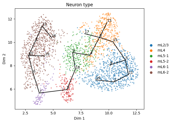
st2.tl.seed_graph(adata,n_clusters=20)
st2.pl.graph(adata,show_text=True,alpha=0.6,color=['Neuron type'],key='seed_epg')
Seeding initial graph...
Clustering...
K-Means clustering ...
Calculating minimum spanning tree...
If the seeded graph does not follow the path we want, we can supervise graph initialization with labels and paths to favor or disfavor (paths_favored, paths_disfavored) with a given strength (label_strength)
[16]:
st2.tl.seed_graph(adata,n_clusters=20,
                  label='Neuron type',
                  label_strength=2.,
                  paths_disfavored=[['mL5-1','mL6-2']],
                 )
st2.pl.graph(adata,show_text=True,alpha=0.6,color=['Neuron type'],key='seed_epg')
Seeding initial graph...
Clustering...
K-Means clustering ...
Calculating minimum spanning tree...

Here we could have achieved the same using paths_favored instead
[17]:
st2.tl.seed_graph(adata,n_clusters=20,
                  label='Neuron type',
                  label_strength=2.,
                  paths_favored=[['mL5-2','mL6-1']],
                 )
st2.pl.graph(adata,show_text=True,alpha=0.6,color=['Neuron type'],key='seed_epg')
Seeding initial graph...
Clustering...
K-Means clustering ...
Calculating minimum spanning tree...
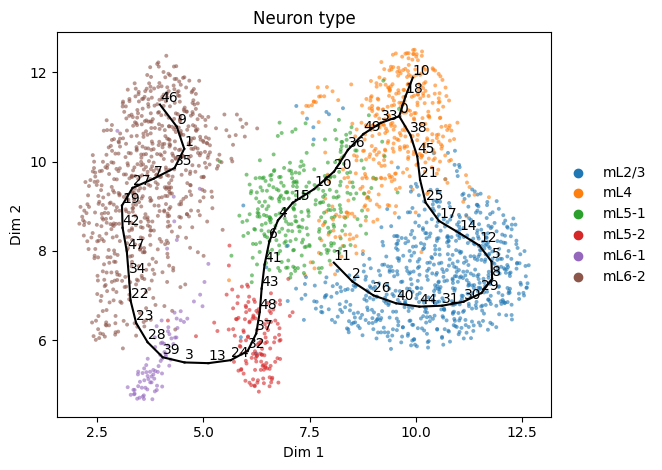
We now refine the seed graph and turn it into a principal graph
[18]:
st2.tl.learn_graph(adata,use_seed=True,verbose=True)
Constructing tree 1 of 1 / Subset 1 of 1
Computing EPG with  50  nodes on  2278  points and  2  dimensions

BARCODE ENERGY  NNODES  NEDGES  NRIBS   NSTARS  NRAYS   NRAYS2  MSE     MSEP    FVE     FVEP    UE      UR      URN     URN2    URSD

3||21   0.9472  21      20      13      3       0       0       0.6047  0.5356  0.9504  0.956   0.2221  0.1204  2.5289  53.1059 0
2||22   0.8878  22      21      16      2       0       0       0.5984  0.5342  0.9509  0.9561  0.2027  0.0867  1.9067  41.9484 0
1||23   0.8284  23      22      19      1       0       0       0.5802  0.52    0.9524  0.9573  0.1885  0.0597  1.373   31.5779 0
1||24   0.812   24      23      20      1       0       0       0.5655  0.5083  0.9536  0.9583  0.1859  0.0607  1.4562  34.9481 0
1||25   0.7908  25      24      21      1       0       0       0.5524  0.4971  0.9547  0.9592  0.1828  0.0556  1.3892  34.7305 0
1||26   0.7767  26      25      22      1       0       0       0.5438  0.4937  0.9554  0.9595  0.1773  0.0556  1.4467  37.6136 0
1||27   0.7606  27      26      23      1       0       0       0.5312  0.4833  0.9564  0.9603  0.1762  0.0533  1.4382  38.8327 0
1||28   0.741   28      27      24      1       0       0       0.5222  0.4763  0.9571  0.9609  0.1718  0.047   1.3162  36.8534 0
1||29   0.7285  29      28      25      1       0       0       0.5143  0.4712  0.9578  0.9613  0.1676  0.0466  1.3504  39.1621 0
1||30   0.7178  30      29      26      1       0       0       0.5066  0.4654  0.9584  0.9618  0.1657  0.0456  1.3665  40.9958 0
1||31   0.7005  31      30      27      1       0       0       0.4953  0.4561  0.9593  0.9626  0.1638  0.0413  1.2814  39.7225 0
1||32   0.6845  32      31      28      1       0       0       0.4856  0.4475  0.9601  0.9633  0.1613  0.0377  1.2051  38.5647 0
1||33   0.6779  33      32      29      1       0       0       0.4818  0.4454  0.9604  0.9634  0.1582  0.0379  1.252   41.3169 0
1||34   0.6691  34      33      30      1       0       0       0.4782  0.4436  0.9607  0.9636  0.1532  0.0377  1.2835  43.6388 0
1||35   0.6557  35      34      31      1       0       0       0.4674  0.4366  0.9616  0.9642  0.1508  0.0376  1.3144  46.0055 0
1||36   0.6429  36      35      32      1       0       0       0.46    0.4294  0.9622  0.9648  0.1489  0.034   1.2244  44.0791 0
1||37   0.6346  37      36      33      1       0       0       0.4529  0.4238  0.9628  0.9652  0.1475  0.0341  1.2626  46.7144 0
1||38   0.6197  38      37      34      1       0       0       0.4415  0.4133  0.9638  0.9661  0.1477  0.0305  1.1596  44.0639 0
1||39   0.6122  39      38      35      1       0       0       0.4366  0.4095  0.9642  0.9664  0.1456  0.03    1.1685  45.5704 0
1||40   0.6057  40      39      36      1       0       0       0.4332  0.4061  0.9644  0.9667  0.1438  0.0287  1.1464  45.8548 0
1||41   0.5951  41      40      37      1       0       0       0.4227  0.3982  0.9653  0.9673  0.1417  0.0307  1.2576  51.5621 0
1||42   0.5877  42      41      38      1       0       0       0.4124  0.3884  0.9662  0.9681  0.1416  0.0338  1.4184  59.5729 0
1||43   0.5862  43      42      39      1       0       0       0.4094  0.3857  0.9664  0.9683  0.1391  0.0377  1.6221  69.7483 0
1||44   0.5749  44      43      40      1       0       0       0.4007  0.3773  0.9671  0.969   0.1394  0.0349  1.5334  67.4714 0
1||45   0.5693  45      44      41      1       0       0       0.3962  0.3739  0.9675  0.9693  0.1367  0.0364  1.6385  73.7308 0
1||46   0.56    46      45      42      1       0       0       0.3875  0.3663  0.9682  0.9699  0.136   0.0365  1.6774  77.1615 0
1||47   0.5521  47      46      43      1       0       0       0.3801  0.3593  0.9688  0.9705  0.1361  0.036   1.6921  79.5296 0
1||48   0.5467  48      47      44      1       0       0       0.3777  0.3578  0.969   0.9706  0.1338  0.0352  1.688   81.0217 0
1||49   0.5395  49      48      45      1       0       0       0.3715  0.3522  0.9695  0.9711  0.1326  0.0354  1.7358  85.055  0
1||50   0.5322  50      49      46      1       0       0       0.3649  0.3459  0.97    0.9716  0.1328  0.0346  1.728   86.4022 0
31.1718  seconds elapsed
[19]:
st2.pl.graph(adata,show_text=True,alpha=0.6,color=['Neuron type'])
Fine-tuning graphs
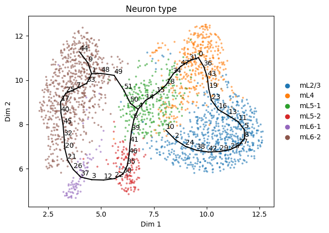
We can further fine-tune the graph by deleting an unwanted branch/path between nodes
[20]:
st2.tl.del_path(adata,0,10)
st2.pl.graph(adata,show_text=True,alpha=0.6,color=['Neuron type'])

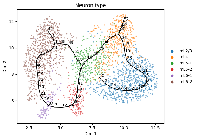
We can also fine-tune the graph by adding a path between nodes
[21]:
st2.tl.add_path(adata,4,1,n_nodes=None)
st2.pl.graph(adata,show_text=True,alpha=0.6,color=['Neuron type'])
Or a path between a node and specified coordinates
[22]:
st2.tl.add_path(adata,0,[10,12],n_nodes=None,epg_mu=1)
st2.pl.graph(adata,show_text=True,alpha=0.6,color=['Neuron type'])
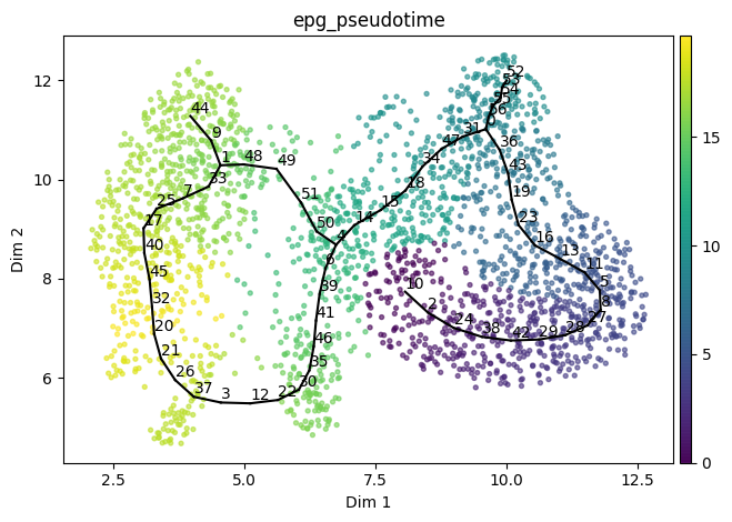
We now compute the pseudotime given a root node
[23]:
st2.tl.infer_pseudotime(adata,source=10,key='epg')
st2.pl.graph(adata,show_text=True,alpha=0.6,color=['epg_pseudotime'])
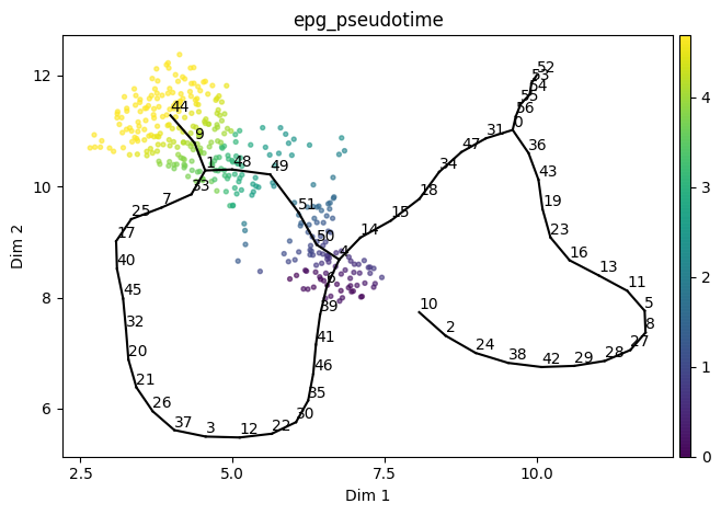
We can also compute the pseudotime for a given path and specify nodes to include in the path
[24]:
st2.tl.infer_pseudotime(adata,source=6,target=44,key='epg')
st2.pl.graph(adata,show_text=True,alpha=0.6,color=['epg_pseudotime'])
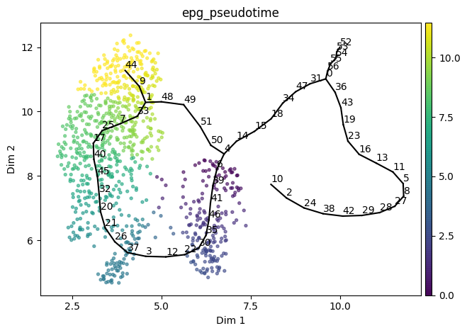
If we wanted to compute pseudotime for the path from above instead, we can specify nodes to include in the path
[25]:
st2.tl.infer_pseudotime(adata,source=6,target=44,nodes_to_include=[25],key='epg')
st2.pl.graph(adata,show_text=True,alpha=0.6,color=['epg_pseudotime'])
[ ]: