multiomics
[ ]:
[1]:
#!pip install muon scanpy hvplot statsmodels scikit-learn
[7]:
pip install -e ../../STREAM2/
Obtaining file:///mnt/c/Users/jobac/Desktop/all/git/STREAM2
  Preparing metadata (setup.py) ... done
Requirement already satisfied: numpy>=1.17.0 in /home/jo/anaconda3/envs/stream2/lib/python3.8/site-packages (from stream2==0.1a0) (1.23.5)
Requirement already satisfied: numba>=0.52.0 in /home/jo/anaconda3/envs/stream2/lib/python3.8/site-packages (from stream2==0.1a0) (0.52.0)
Requirement already satisfied: networkx>=2.5 in /home/jo/anaconda3/envs/stream2/lib/python3.8/site-packages (from stream2==0.1a0) (3.1)
Requirement already satisfied: pandas!=1.1,>=1.0 in /home/jo/.local/lib/python3.8/site-packages (from stream2==0.1a0) (1.3.5)
Requirement already satisfied: anndata>=0.7.4 in /home/jo/anaconda3/envs/stream2/lib/python3.8/site-packages (from stream2==0.1a0) (0.8.0)
Requirement already satisfied: scanpy>=1.6.0 in /home/jo/anaconda3/envs/stream2/lib/python3.8/site-packages (from stream2==0.1a0) (1.9.3)
Requirement already satisfied: shapely>=2.0.1 in /home/jo/anaconda3/envs/stream2/lib/python3.8/site-packages (from stream2==0.1a0) (2.0.1)
Requirement already satisfied: statsmodels>=0.12.1 in /home/jo/anaconda3/envs/stream2/lib/python3.8/site-packages (from stream2==0.1a0) (0.13.5)
Requirement already satisfied: scikit-learn>=1.2 in /home/jo/anaconda3/envs/stream2/lib/python3.8/site-packages (from stream2==0.1a0) (1.2.2)
Requirement already satisfied: scipy>=1.4 in /home/jo/anaconda3/envs/stream2/lib/python3.8/site-packages (from stream2==0.1a0) (1.10.1)
Requirement already satisfied: kneed>=0.7 in /home/jo/anaconda3/envs/stream2/lib/python3.8/site-packages (from stream2==0.1a0) (0.7.0)
Requirement already satisfied: seaborn>=0.11 in /home/jo/anaconda3/envs/stream2/lib/python3.8/site-packages (from stream2==0.1a0) (0.12.2)
Requirement already satisfied: matplotlib>=3.3 in /home/jo/anaconda3/envs/stream2/lib/python3.8/site-packages (from stream2==0.1a0) (3.7.1)
Requirement already satisfied: plotly>=4.14.0 in /home/jo/anaconda3/envs/stream2/lib/python3.8/site-packages (from stream2==0.1a0) (5.14.1)
Requirement already satisfied: scikit-misc>=0.1.3 in /home/jo/anaconda3/envs/stream2/lib/python3.8/site-packages (from stream2==0.1a0) (0.2.0)
Requirement already satisfied: adjusttext>=0.7.3 in /home/jo/anaconda3/envs/stream2/lib/python3.8/site-packages (from stream2==0.1a0) (0.8)
Requirement already satisfied: umap-learn>=0.4.6 in /home/jo/anaconda3/envs/stream2/lib/python3.8/site-packages (from stream2==0.1a0) (0.5.3)
Requirement already satisfied: elpigraph-python>=0.3.1 in /home/jo/anaconda3/envs/stream2/lib/python3.8/site-packages (from stream2==0.1a0) (0.3.1)
Requirement already satisfied: python-slugify>=5.0.0 in /home/jo/anaconda3/envs/stream2/lib/python3.8/site-packages (from stream2==0.1a0) (8.0.1)
Requirement already satisfied: h5py>=3 in /home/jo/anaconda3/envs/stream2/lib/python3.8/site-packages (from anndata>=0.7.4->stream2==0.1a0) (3.8.0)
Requirement already satisfied: natsort in /home/jo/anaconda3/envs/stream2/lib/python3.8/site-packages (from anndata>=0.7.4->stream2==0.1a0) (8.3.1)
Requirement already satisfied: packaging>=20 in /home/jo/anaconda3/envs/stream2/lib/python3.8/site-packages (from anndata>=0.7.4->stream2==0.1a0) (23.1)
Requirement already satisfied: python-igraph>=0.7.1 in /home/jo/anaconda3/envs/stream2/lib/python3.8/site-packages (from elpigraph-python>=0.3.1->stream2==0.1a0) (0.10.4)
Requirement already satisfied: contourpy>=1.0.1 in /home/jo/anaconda3/envs/stream2/lib/python3.8/site-packages (from matplotlib>=3.3->stream2==0.1a0) (1.0.7)
Requirement already satisfied: cycler>=0.10 in /home/jo/anaconda3/envs/stream2/lib/python3.8/site-packages (from matplotlib>=3.3->stream2==0.1a0) (0.11.0)
Requirement already satisfied: fonttools>=4.22.0 in /home/jo/anaconda3/envs/stream2/lib/python3.8/site-packages (from matplotlib>=3.3->stream2==0.1a0) (4.39.3)
Requirement already satisfied: kiwisolver>=1.0.1 in /home/jo/anaconda3/envs/stream2/lib/python3.8/site-packages (from matplotlib>=3.3->stream2==0.1a0) (1.4.4)
Requirement already satisfied: pillow>=6.2.0 in /home/jo/anaconda3/envs/stream2/lib/python3.8/site-packages (from matplotlib>=3.3->stream2==0.1a0) (9.4.0)
Requirement already satisfied: pyparsing>=2.3.1 in /home/jo/anaconda3/envs/stream2/lib/python3.8/site-packages (from matplotlib>=3.3->stream2==0.1a0) (3.0.9)
Requirement already satisfied: python-dateutil>=2.7 in /home/jo/anaconda3/envs/stream2/lib/python3.8/site-packages (from matplotlib>=3.3->stream2==0.1a0) (2.8.2)
Requirement already satisfied: importlib-resources>=3.2.0 in /home/jo/anaconda3/envs/stream2/lib/python3.8/site-packages (from matplotlib>=3.3->stream2==0.1a0) (5.12.0)
Requirement already satisfied: llvmlite<0.36,>=0.35.0 in /home/jo/anaconda3/envs/stream2/lib/python3.8/site-packages (from numba>=0.52.0->stream2==0.1a0) (0.35.0)
Requirement already satisfied: setuptools in /home/jo/anaconda3/envs/stream2/lib/python3.8/site-packages (from numba>=0.52.0->stream2==0.1a0) (67.6.1)
Requirement already satisfied: pytz>=2017.3 in /home/jo/anaconda3/envs/stream2/lib/python3.8/site-packages (from pandas!=1.1,>=1.0->stream2==0.1a0) (2023.3)
Requirement already satisfied: tenacity>=6.2.0 in /home/jo/anaconda3/envs/stream2/lib/python3.8/site-packages (from plotly>=4.14.0->stream2==0.1a0) (8.2.2)
Requirement already satisfied: text-unidecode>=1.3 in /home/jo/anaconda3/envs/stream2/lib/python3.8/site-packages (from python-slugify>=5.0.0->stream2==0.1a0) (1.3)
Requirement already satisfied: tqdm in /home/jo/anaconda3/envs/stream2/lib/python3.8/site-packages (from scanpy>=1.6.0->stream2==0.1a0) (4.65.0)
Requirement already satisfied: patsy in /home/jo/anaconda3/envs/stream2/lib/python3.8/site-packages (from scanpy>=1.6.0->stream2==0.1a0) (0.5.3)
Requirement already satisfied: joblib in /home/jo/anaconda3/envs/stream2/lib/python3.8/site-packages (from scanpy>=1.6.0->stream2==0.1a0) (1.2.0)
Requirement already satisfied: session-info in /home/jo/anaconda3/envs/stream2/lib/python3.8/site-packages (from scanpy>=1.6.0->stream2==0.1a0) (1.0.0)
Requirement already satisfied: threadpoolctl>=2.0.0 in /home/jo/anaconda3/envs/stream2/lib/python3.8/site-packages (from scikit-learn>=1.2->stream2==0.1a0) (3.1.0)
Requirement already satisfied: pynndescent>=0.5 in /home/jo/anaconda3/envs/stream2/lib/python3.8/site-packages (from umap-learn>=0.4.6->stream2==0.1a0) (0.5.10)
Requirement already satisfied: zipp>=3.1.0 in /home/jo/anaconda3/envs/stream2/lib/python3.8/site-packages (from importlib-resources>=3.2.0->matplotlib>=3.3->stream2==0.1a0) (3.15.0)
Requirement already satisfied: six in /home/jo/anaconda3/envs/stream2/lib/python3.8/site-packages (from patsy->scanpy>=1.6.0->stream2==0.1a0) (1.16.0)
Requirement already satisfied: igraph==0.10.4 in /home/jo/anaconda3/envs/stream2/lib/python3.8/site-packages (from python-igraph>=0.7.1->elpigraph-python>=0.3.1->stream2==0.1a0) (0.10.4)
Requirement already satisfied: texttable>=1.6.2 in /home/jo/anaconda3/envs/stream2/lib/python3.8/site-packages (from igraph==0.10.4->python-igraph>=0.7.1->elpigraph-python>=0.3.1->stream2==0.1a0) (1.6.7)
Requirement already satisfied: stdlib-list in /home/jo/anaconda3/envs/stream2/lib/python3.8/site-packages (from session-info->scanpy>=1.6.0->stream2==0.1a0) (0.8.0)
Installing collected packages: stream2
  Attempting uninstall: stream2
    Found existing installation: stream2 0.1a0
    Uninstalling stream2-0.1a0:
      Successfully uninstalled stream2-0.1a0
  Running setup.py develop for stream2
Successfully installed stream2-0.1a0
Note: you may need to restart the kernel to use updated packages.
[1]:
import scanpy as sc
import muon as mu
import stream2 as st2

import numpy as np
import pandas as pd
import seaborn as sns
import matplotlib.pyplot as plt
import hvplot.pandas
from session_info import show
show()
/home/jo/anaconda3/envs/stream2/lib/python3.8/site-packages/tqdm/auto.py:21: TqdmWarning: IProgress not found. Please update jupyter and ipywidgets. See https://ipywidgets.readthedocs.io/en/stable/user_install.html
  from .autonotebook import tqdm as notebook_tqdm
---------------------------------------------------------------------------
KeyError                                  Traceback (most recent call last)
Cell In[1], line 11
      9 import hvplot.pandas
     10 from session_info import show
---> 11 show()

File ~/anaconda3/envs/stream2/lib/python3.8/site-packages/session_info/main.py:209, in show(na, os, cpu, jupyter, dependencies, std_lib, private, write_req_file, req_file_name, html, excludes)
    207 for mod_name in clean_modules:
    208     mod_names.append(mod_name)
--> 209     mod = sys.modules[mod_name]
    210     # Since modules use different attribute names to store version info,
    211     # try the most common ones.
    212     try:

KeyError: 'cupy'
Multi-modal trajectory inference demo
We load four assays (two scATAC and two scRNA) integrated into one anndata object.
adata_integrated.X contains gene expression (gene scores for ATAC cells) for 200 highly variable genes.
We will use this subset of measurements from hematopoietic cells as a toy example.
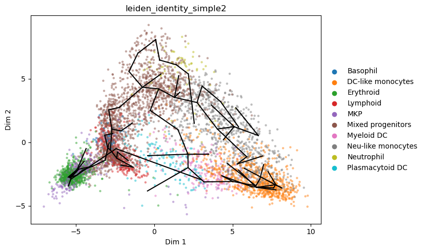
[2]:
adata_integrated = st2.read_h5ad('../data/multiomics/atac_rna_toy200.h5ad')
#sc.pp.neighbors(adata_integrated,n_neighbors=50,metric='cosine',use_rep='X_pca_transp_emd')
#sc.tl.umap(adata_integrated,min_dist=0.05)
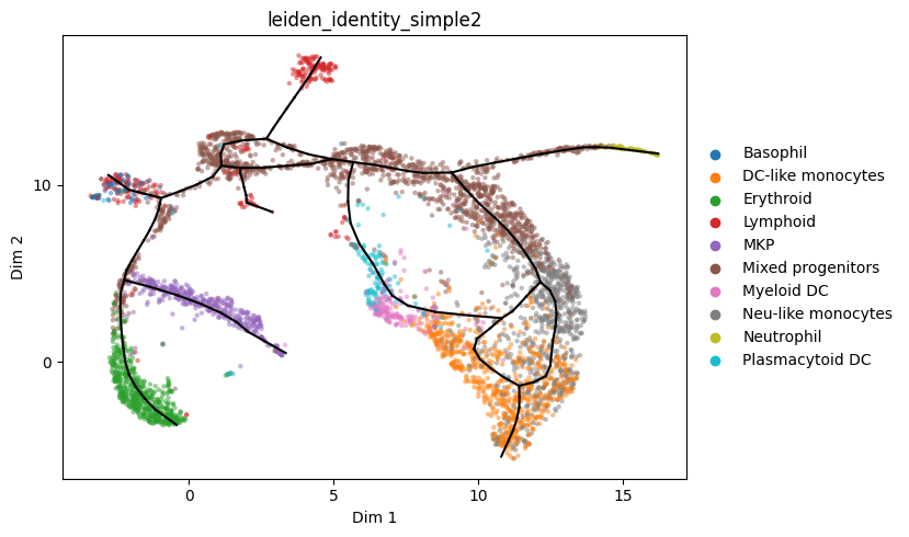
sc.pl.umap(adata_integrated[::-1],color=['assay_detailed','leiden_identity_simple2',],wspace=.2)
/home/jo/anaconda3/envs/stream2/lib/python3.8/site-packages/anndata/compat/_overloaded_dict.py:106: ImplicitModificationWarning: Trying to modify attribute `._uns` of view, initializing view as actual.
  self.data[key] = value
/home/jo/anaconda3/envs/stream2/lib/python3.8/site-packages/scanpy/plotting/_tools/scatterplots.py:392: UserWarning: No data for colormapping provided via 'c'. Parameters 'cmap' will be ignored
  cax = scatter(
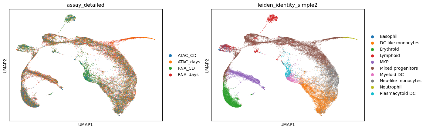
In this case we have 4 assays with same features (since we only loaded gene scores for ATAC), which fits nicely into a single anndata.
However in general it is not possible to simply concatenate assays with possibly different features and observations into a single anndata.
The solution is to use the muon package and its MuData format to store our multimodal assays
[3]:
assays = adata_integrated.obs['assay_detailed']
adatas = {assay: adata_integrated[assays==assay] for assay in assays.unique()}
mdata = mu.MuData(adatas)
mdata
/home/jo/anaconda3/envs/stream2/lib/python3.8/site-packages/mudata/_core/mudata.py:457: UserWarning: Cannot join columns with the same name because var_names are intersecting.
  warnings.warn(
[3]:
MuData object with n_obs × n_vars = 99955 × 800
  4 modalities
    ATAC_CD:        13575 x 200
      obs:  'leiden_identity_simple2', 'label', 'assay_detailed'
      obsm: 'X_pca_transp_emd', 'X_umap'
    ATAC_days:      19206 x 200
      obs:  'leiden_identity_simple2', 'label', 'assay_detailed'
      obsm: 'X_pca_transp_emd', 'X_umap'
    RNA_CD: 22804 x 200
      obs:  'leiden_identity_simple2', 'label', 'assay_detailed'
      obsm: 'X_pca_transp_emd', 'X_umap'
    RNA_days:       44370 x 200
      obs:  'leiden_identity_simple2', 'label', 'assay_detailed'
      obsm: 'X_pca_transp_emd', 'X_umap'
In our case cells are not matched between assays so we had to perform data integration to get a joint UMAP representation We will learn a joint trajectory based on this joint representation. Let’s store it along with cell annotation at the global rather than assay level in mdata
[4]:
mdata.obsm['X_dr'] = mdata.obsm['X_umap'] = np.vstack([adata.obsm['X_umap'] for adata in mdata.mod.values()])
mdata.obsm['X_pca_transp_emd'] = np.vstack([adata.obsm['X_pca_transp_emd'] for adata in mdata.mod.values()])
mdata.obs['leiden_identity_simple2'] = np.hstack([adata.obs['leiden_identity_simple2'] for adata in mdata.mod.values()])
If your data contains matched cells, you have more choice and can learn the trajectory based on: - some RNA representation - some ATAC representation - some joint RNA+ATAC representation obtained using your favorite method e.g.: - MOFA (mu.tl.mofa(mdata)) - J-UMAP https://github.com/canzarlab/JVis-learn - UMAP tutorial for multiple views https://umap-learn.readthedocs.io/en/latest/composing_models.html
If your data contains non-matched cells then assays can be integrated into a joint representation. Some suggestions of methods to obtain it: - Harmony, Scanorama (scanpy.pp.external) - Optimal transport https://pythonot.github.io/ - Joint MDS https://github.com/BorgwardtLab/JointMDS - MultiMAP https://github.com/Teichlab/MultiMAP
Let’s work with a subsample (just to speed up trajectory inference, it’s also fine to use mdata directly)
[5]:
idx = np.random.RandomState(0).choice(mdata.shape[0],5000,replace=False)

a_s = sc.AnnData(np.zeros((5000,1)))
a_s.obsm['X_pca_transp_emd'] = mdata.obsm['X_pca_transp_emd'][idx]
a_s.obsm['X_dr'] = a_s.obsm['X_umap'] = mdata.obsm['X_umap'][idx]
a_s.obs['leiden_identity_simple2'] = mdata.obs['leiden_identity_simple2'][idx].values
/tmp/ipykernel_2000/1930611853.py:3: FutureWarning: X.dtype being converted to np.float32 from float64. In the next version of anndata (0.9) conversion will not be automatic. Pass dtype explicitly to avoid this warning. Pass `AnnData(X, dtype=X.dtype, ...)` to get the future behavour.
  a_s = sc.AnnData(np.zeros((5000,1)))
Trajectory inference in 2d
We will first illustrate how to learn a trajectory in 2D before illustrating higher dimensions.
We seed graph with a minimum spanning tree. Forbid the tree to form paths connecting Neu-like to DC-like monocytes
[12]:
st2.tl.seed_graph(a_s,n_clusters=80, label_strength=2.5,
                  paths_disfavored=[['Neu-like monocytes','DC-like monocytes']],label='leiden_identity_simple2')
st2.pl.graph(a_s,color=['leiden_identity_simple2'],alpha=.5,size=10,fig_size=(8,5),key='seed_epg')
Seeding initial graph...
Clustering...
K-Means clustering ...
Calculating minimum spanning tree...
/mnt/c/Users/jobac/Desktop/all/git/STREAM2/stream2/tools/_elpigraph.py:865: FutureWarning: Unlike other reduction functions (e.g. `skew`, `kurtosis`), the default behavior of `mode` typically preserves the axis it acts along. In SciPy 1.11.0, this behavior will change: the default value of `keepdims` will become False, the `axis` over which the statistic is taken will be eliminated, and the value None will no longer be accepted. Set `keepdims` to True or False to avoid this warning.
  modes[i] = scipy.stats.mode(labels[part == i]).mode[0]
/home/jo/anaconda3/envs/stream2/lib/python3.8/site-packages/scipy/stats/_stats_py.py:112: RuntimeWarning: The input array could not be properly checked for nan values. nan values will be ignored.
  warnings.warn("The input array could not be properly "
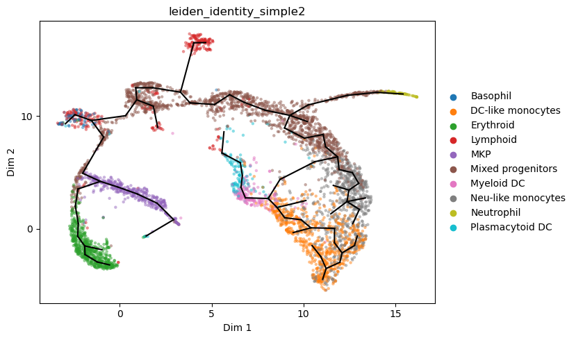
We refine the graph.
We speed up computations by limiting the max number of candidate graphs considered when fitting.
We emphasize less dense regions with slightly higher point weights
[13]:
st2.tl.get_weights(a_s,bandwidth=2)
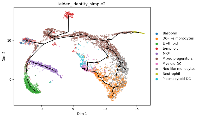
st2.tl.learn_graph(a_s,n_nodes=95,epg_lambda=0.02,epg_mu=0.05,epg_alpha=0.02,use_weights=True,verbose=1,
max_candidates = {"AddNode2Node": 10,"BisectEdge": 10,"ShrinkEdge": 0,})
st2.pl.graph(a_s,color=['leiden_identity_simple2'],alpha=.5,size=10,fig_size=(10,6))
Constructing tree 1 of 1 / Subset 1 of 1
Computing EPG with  95  nodes on  5000  points and  2  dimensions

BARCODE ENERGY  NNODES  NEDGES  NRIBS   NSTARS  NRAYS   NRAYS2  MSE     MSEP    FVE     FVEP    UE      UR      URN     URN2    URSD

1|13||81        1.8126  81      80      50      13      0       0       0.504   0.454   0.9915  0.9924  1.2937  0.0148  1.1968  96.9448 0
1|12||82        1.7496  82      81      53      12      0       0       0.5022  0.4546  0.9916  0.9924  1.2332  0.0143  1.1693  95.8848 0
1|11||83        1.6986  83      82      56      11      0       0       0.5013  0.4559  0.9916  0.9923  1.1829  0.0144  1.1959  99.2564 0
12||84  1.6596  84      83      58      12      0       0       0.492   0.4479  0.9917  0.9925  1.1546  0.0131  1.0982  92.2525 0
11||85  1.6202  85      84      61      11      0       0       0.4905  0.4492  0.9918  0.9925  1.1164  0.0133  1.1298  96.0343 0
10||86  1.5849  86      85      64      10      0       0       0.4853  0.4457  0.9918  0.9925  1.0868  0.0128  1.1006  94.6513 0
9||87   1.5572  87      86      67      9       0       0       0.4834  0.4453  0.9919  0.9925  1.0609  0.0129  1.1238  97.7669 0
9||88   1.5259  88      87      68      9       0       0       0.4748  0.438   0.992   0.9926  1.0391  0.0119  1.046   92.046  0
8||89   1.4977  89      88      71      8       0       0       0.4675  0.432   0.9921  0.9927  1.019   0.0112  0.9961  88.656  0
8||90   1.4824  90      89      72      8       0       0       0.4763  0.4411  0.992   0.9926  0.9918  0.0143  1.2884  115.9605        0
7||91   1.4582  91      90      75      7       0       0       0.4765  0.4426  0.992   0.9926  0.9693  0.0124  1.1254  102.415 0
7||92   1.4527  92      91      76      7       0       0       0.4855  0.453   0.9918  0.9924  0.9506  0.0166  1.5287  140.639 0
7||93   1.4382  93      92      77      7       0       0       0.4822  0.4507  0.9919  0.9924  0.9394  0.0166  1.5483  143.9908        0
7||94   1.4305  94      93      78      7       0       0       0.4874  0.456   0.9918  0.9923  0.9256  0.0175  1.6493  155.031 0
7||95   1.417   95      94      79      7       0       0       0.4883  0.4581  0.9918  0.9923  0.9113  0.0173  1.6421  156.0022        0
36.4012  seconds elapsed
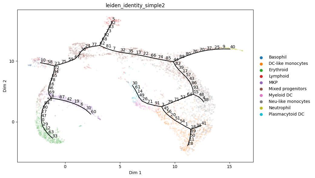
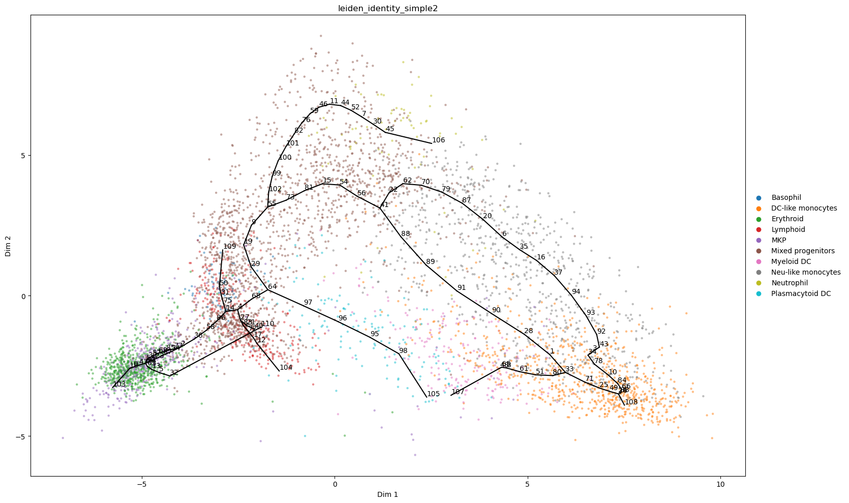
Visualize node labels
[10]:
st2.pl.graph(a_s,color=['leiden_identity_simple2'],alpha=.1,size=10,fig_size=(10,6),show_text=1)
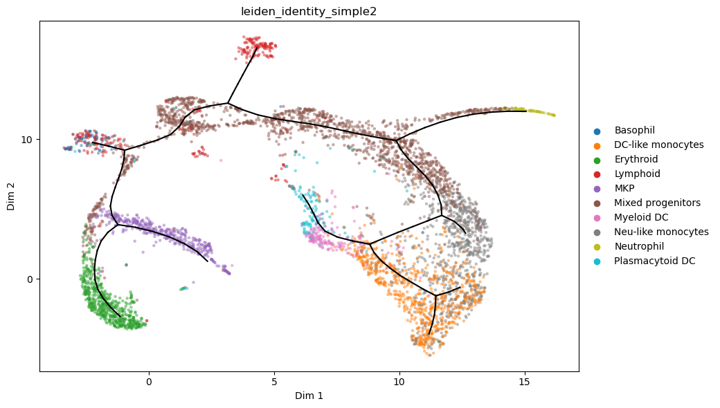
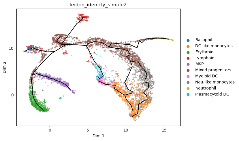
Fine tune the graph by: - adding extra plausible paths - refitting the graph while forcing some nodes to remain fixed at chosen positions - extending leaves so branches reach the end of the distribution
[11]:
a_s2 = a_s.copy()

st2.tl.add_path(a_s2,38,41,refit_graph=True,use_weights=True)

st2.tl.refit_graph(a_s2,shift_nodes_pos={
    3 : a_s2.uns['epg']['node_pos'][3] + np.array([+2, +0]),
    24 : a_s2.uns['epg']['node_pos'][24] + np.array([-.6, +.2]),
    25 : a_s2.uns['epg']['node_pos'][25] + np.array([+0., +.2]),
    8  : a_s2.uns['epg']['node_pos'][8] + np.array([-1,  +.75]),
    44 : a_s2.uns['epg']['node_pos'][44] + np.array([-.8,+.8]),
    }
)

st2.tl.add_path(a_s2,2,32,epg_lambda=.2)
st2.tl.add_path(a_s2,30,35,epg_lambda=.2,epg_mu=.2)
st2.tl.add_path(a_s2,99,[2.,9.],epg_lambda=.2,epg_mu=.2)
st2.tl.extend_leaves(a_s2,Mode="QuantDists",ControlPar=.75)
st2.pl.graph(a_s2,color=['leiden_identity_simple2'],alpha=.5,size=10,fig_size=(8,5))
Performing simulated annealing. This may take a while
Performing simulated annealing. This may take a while
Performing simulated annealing. This may take a while
Performing simulated annealing. This may take a while
Performing simulated annealing. This may take a while
Performing simulated annealing. This may take a while
Performing simulated annealing. This may take a while
(7, 2)
(112, 2)
Store graph computed on the subsample back to mdata with the full dataset
[16]:
mdata.uns = a_s2.uns.copy()
# this recomputes the projection of cells onto the graph
st2.tl._elpigraph._store_graph_attributes(mdata,mdata.obsm['X_dr'],'epg')
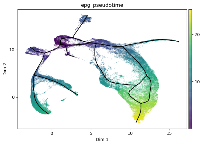
Infer pseudotime for a given root node
[17]:
st2.tl.infer_pseudotime(mdata,source=2)
st2.pl.graph(mdata,color=['epg_pseudotime'],size=.1,alpha=.3)
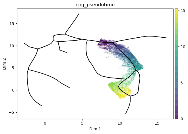
Infer pseudotime for a given path
[18]:
st2.tl.infer_pseudotime(mdata,source=66,target=1)
st2.pl.graph(mdata,color=['epg_pseudotime'],size=.1,alpha=.3)
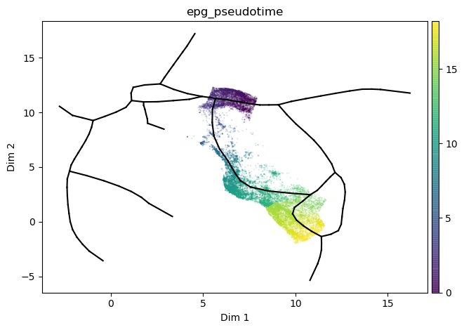
Use nodes_to_include to take a longer path rather than the shortest (default)
[19]:
st2.tl.infer_pseudotime(mdata,source=66,target=1,nodes_to_include=[26])
st2.pl.graph(mdata,color=['epg_pseudotime'],size=.1,alpha=.3)
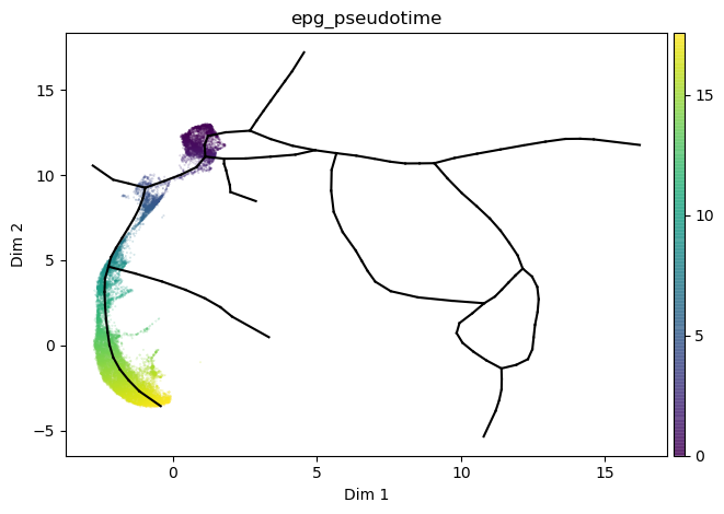
Let’s investigate Erythroids. We compute transition markers (that go up or down along the path) for each assay separately
method = ‘spearman’ for spearman correlation
method = ‘xi’ for non-linear XI correlation, returns values between 0-1
[20]:
source, target = 24, 115

st2.tl.infer_pseudotime(mdata,source=24,target=115)
st2.pl.graph(mdata,color=['epg_pseudotime'],size=.1,alpha=.3)

transition_markers = {}
for assay,adata in mdata.mod.items():
    adata.uns['epg']=mdata.uns['epg']
    adata.obs = adata.obs.join(mdata.obs[[k for k in mdata.obs if 'epg' in k]])
    st2.tl.infer_pseudotime(adata,source=24,target=115)
    st2.tl.detect_transition_markers(adata,fc_cutoff=0., method='spearman')

    transition_markers[assay] = adata.uns['transition_markers'][f'Path_{source}-None-{target}']
/home/jo/anaconda3/envs/stream2/lib/python3.8/site-packages/anndata/compat/_overloaded_dict.py:106: ImplicitModificationWarning: Trying to modify attribute `._uns` of view, initializing view as actual.
  self.data[key] = value
2905 Cells are selected for Path_Source_Nodes-to-include_Target :  Path_24-None-115
Filtering out markers that are expressed in less than 5 cells ...
200 markers are being scanned ...
/home/jo/anaconda3/envs/stream2/lib/python3.8/site-packages/anndata/compat/_overloaded_dict.py:106: ImplicitModificationWarning: Trying to modify attribute `._uns` of view, initializing view as actual.
  self.data[key] = value
3508 Cells are selected for Path_Source_Nodes-to-include_Target :  Path_24-None-115
Filtering out markers that are expressed in less than 5 cells ...
200 markers are being scanned ...
3993 Cells are selected for Path_Source_Nodes-to-include_Target :  Path_24-None-115
Filtering out markers that are expressed in less than 5 cells ...
200 markers are being scanned ...
9514 Cells are selected for Path_Source_Nodes-to-include_Target :  Path_24-None-115
Filtering out markers that are expressed in less than 5 cells ...
200 markers are being scanned ...
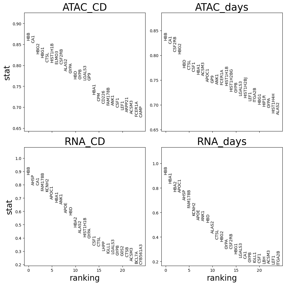
Plot results
[21]:
def plot_top_markers(transition_markers,sort_by = 'logfc',n_genes = 25):

    f,axs=plt.subplots(2,2,figsize=(10,10),sharex=True)
    axs=axs.flat
    for i,n in zip(range(len(transition_markers)),transition_markers.keys()):

        # get data
        df = transition_markers[n][sort_by].sort_values()[::-1][:n_genes]
        gene_names, scores = df.index, df.values

        # plot
        ymax, ymin = np.max(scores), np.min(scores) - 0.05*np.min(scores)
        ymax += 0.3 * (ymax - ymin)

        ax=next(axs)
        ax.set_ylim(ymin, ymax)
        ax.set_xlim(-0.9, n_genes - 0.1)
        ax.set_title(n,fontsize=25)
        if i>1: ax.set_xlabel('ranking',fontsize=20)
        if i==0 or i==2: ax.set_ylabel(sort_by,fontsize=20)

        # Making labels
        for ig, gene_name in enumerate(gene_names):
            ax.text(ig,scores[ig],gene_name,rotation='vertical',verticalalignment='bottom',horizontalalignment='center',fontsize=10,)
    plt.tight_layout(); plt.show()


plot_top_markers(transition_markers, sort_by = 'stat',n_genes = 25,)

df = pd.concat(transition_markers).reset_index().rename(columns={'level_0':'assay_detailed','level_1':'var_names'})
df.hvplot.scatter("stat", "logfc", flip_yaxis=False, logy=False, by='assay_detailed',hover_cols=["var_names"],height=500,width=800)
[21]:
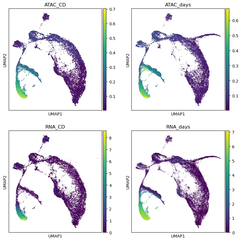
Let’s check some of those markers found in several assays
[22]:
def scatterplot_assays(color):
    f,axs=plt.subplots(2,2,figsize=(10,10),sharex=True)
    axs=axs.flat
    for assay,adata in mdata.mod.items():
        ax=next(axs)
        sc.pl.umap(adata,color=color,ax=ax,show=False)
        ax.set_title(assay)
    plt.show()

scatterplot_assays('HBB')
We can try to correlate assays’ variables directly.
In our case cells are not matched across assays; this means they will have different pseudotime values
To deal with this a simple approach is to interpolate data and resample at the same pseudotime values. If your cells are matched you don’t need this step
[23]:
import scipy

interpolated = {}
for assay, adata in mdata.mod.items():
    #arrays need to be dense for this step
    if scipy.sparse.issparse(adata.X):
        adata.X=adata.X.toarray()
    interpolated[assay] = st2.tl.interpolate(adata,t_len=200,method='knn',frac=.1,n_neighbors='auto',weights='uniform')[1]
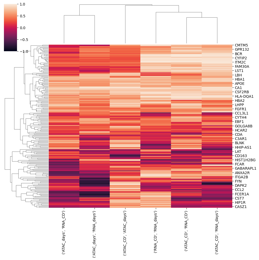
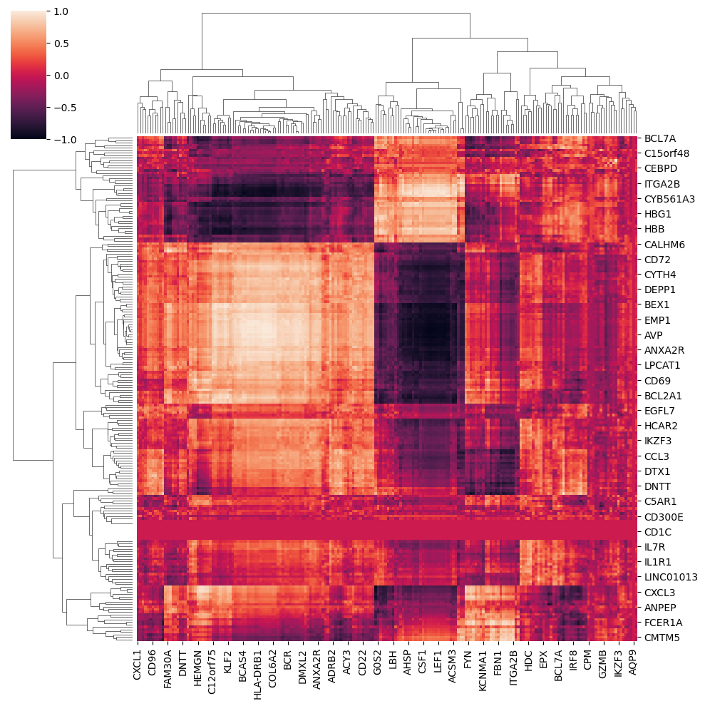
Now that we have data with the same pseudotime values we can correlate variables with same name across assays
[24]:
correlations = {}
modalities = list(mdata.mod.keys())

for i in range(mdata.n_mod-1):
    for j in range(i+1,mdata.n_mod):

        correlations[modalities[i],modalities[j]] = st2.tl.spearman_columns(interpolated[modalities[i]],
                                                                            interpolated[modalities[j]])
                                                   #or st2.tl.xicorr_columns()[0]

correlations = pd.DataFrame(correlations)
correlations.index = mdata[modalities[0]].var_names
correlations.columns = correlations.columns.to_flat_index()
sns.clustermap(correlations.dropna(),vmin=-1,vmax=1)
[24]:
<seaborn.matrix.ClusterGrid at 0x7f6142416970>
If variables were different across assays we could correlate all with all instead
[25]:
correlations_all = {}
modalities = list(mdata.mod.keys())
for i in range(mdata.n_mod-1):
    for j in range(i+1,mdata.n_mod):
        correlations_all[modalities[i],modalities[j]] = st2.tl.spearman_pairwise(interpolated[modalities[i]],
                                                                                 interpolated[modalities[j]])
                                                        #or st2.tl.xicorr_pairwise()[0]


mi,mj = 'RNA_CD','RNA_days'
corrs_all = pd.DataFrame(correlations_all[mi,mj])
corrs_all.index, corrs_all.columns = mdata[mi].var_names, mdata[mj].var_names
corrs_all[corrs_all.isna()]=0.
sns.clustermap(corrs_all,vmin=-1,vmax=1)
/home/jo/anaconda3/envs/stream2/lib/python3.8/site-packages/seaborn/matrix.py:560: UserWarning: Clustering large matrix with scipy. Installing `fastcluster` may give better performance.
  warnings.warn(msg)
[25]:
<seaborn.matrix.ClusterGrid at 0x7f6142c8e160>
Let’s visualize results as scatter plots.
e.g., we can plot spearman correlation against pseudotime for two assays and color by their correlation.
[26]:
def plot_two_assays(transition_markers,mod1, mod2, plot_var='stat',color='dodgerblue',cmap='Viridis'):
    selected = [mod1,mod2]
    selected_dfs = {k:v for k,v in transition_markers.items() if k in selected}
    df = pd.concat(selected_dfs,axis=1,keys=selected).dropna()
    df.columns = df.columns.to_flat_index().map(lambda s:' '.join(s))

    if type(color)!=str:
        df = df.join(color)
        color, clabel = df[color.name], color.name
    else:
        clabel = color

    df.index.name='var_name'
    return df.hvplot.scatter(f'{mod1} {plot_var}',f'{mod2} {plot_var}', hover_cols=["var_name"],
                             color=color,cmap=cmap,clabel=clabel, hover=True,
                             xlim=(-1.05,1.05),ylim=(-1.05,1.05),height=500,width=600)

def compose_fig(plots,ncols=2):
    figure = '('+ '+'.join([f'plots[{i}]' for i in range(len(plots))]) + f').cols({ncols})'
    return eval(figure)

plots = []
for i in range(mdata.n_mod-1):
    for j in range(i+1,mdata.n_mod):
        color = correlations[modalities[i],modalities[j]].rename('correlation '+modalities[i]+' vs '+modalities[j])
        plots.append( plot_two_assays(transition_markers,modalities[i],modalities[j], plot_var='stat', color=color) )

compose_fig(plots,2)
[26]:
Trajectory inference in higher dimension
We now show how the trajectory can be learnt based on the higher dimensional PCA data instead
[27]:
a_s.obsm['X_dr'] = a_s.obsm['X_pca_transp_emd']
st2.tl.seed_graph(a_s,n_clusters=80,label_strength=2.5,paths_disfavored=[['Neu-like monocytes','DC-like monocytes']],label='leiden_identity_simple2')
st2.pl.graph(a_s,color=['leiden_identity_simple2'],alpha=.5,size=10,fig_size=(8,5),key='seed_epg')
Seeding initial graph...
Clustering...
K-Means clustering ...
Calculating minimum spanning tree...
/mnt/c/Users/jobac/Desktop/all/git/STREAM2/stream2/tools/_elpigraph.py:865: FutureWarning: Unlike other reduction functions (e.g. `skew`, `kurtosis`), the default behavior of `mode` typically preserves the axis it acts along. In SciPy 1.11.0, this behavior will change: the default value of `keepdims` will become False, the `axis` over which the statistic is taken will be eliminated, and the value None will no longer be accepted. Set `keepdims` to True or False to avoid this warning.
  modes[i] = scipy.stats.mode(labels[part == i]).mode[0]
/home/jo/anaconda3/envs/stream2/lib/python3.8/site-packages/scipy/stats/_stats_py.py:112: RuntimeWarning: The input array could not be properly checked for nan values. nan values will be ignored.
  warnings.warn("The input array could not be properly "
To make sense of how the graph fits to data, it can be useful to roughly represent its position on the 2D umap rather than PC axes.
We achieve this by projecting data points onto their closest node, and defining 2D node positions as the centroid of their associated points
[28]:
st2.tl.project_graph(a_s, to_basis='X_umap', key='seed_epg')
st2.pl.graph(a_s,color=['leiden_identity_simple2'],alpha=.5,size=10,fig_size=(8,5),key='seed_epg_from_X_dr_to_X_umap')
[29]:
st2.tl.learn_graph(a_s,n_nodes=100,epg_lambda=0.02,epg_mu=0.05,epg_alpha=0.02,verbose=1,store_evolution=True)
                   #max_candidates = {"AddNode2Node": 10,"BisectEdge": 10,"ShrinkEdge": 0,})
st2.pl.graph(a_s,color=['leiden_identity_simple2'],alpha=.5,size=10,fig_size=(8,5))
Constructing tree 1 of 1 / Subset 1 of 1
Computing EPG with  100  nodes on  5000  points and  14  dimensions

BARCODE ENERGY  NNODES  NEDGES  NRIBS   NSTARS  NRAYS   NRAYS2  MSE     MSEP    FVE     FVEP    UE      UR      URN     URN2    URSD

4|17||81        8.6429  81      80      33      17      0       0       6.072   5.9942  0.8758  0.8774  2.5113  0.0597  4.8363  391.7442        0
3|18||82        8.5494  82      81      35      18      0       0       6.0528  5.9804  0.8762  0.8777  2.4401  0.0565  4.637   380.2305        0
2|19||83        8.451   83      82      37      19      0       0       6.0332  5.9652  0.8766  0.878   2.3627  0.0551  4.5701  379.3221        0
1|20||84        8.3884  84      83      39      20      0       0       6.0106  5.9425  0.8771  0.8785  2.321   0.0568  4.7691  400.6011        0
1|19||85        8.3177  85      84      42      19      0       0       5.9905  5.9232  0.8775  0.8788  2.2717  0.0555  4.7141  400.6955        0
20||86  8.2488  86      85      44      20      0       0       5.9737  5.908   0.8778  0.8792  2.2199  0.0552  4.7432  407.9185        0
19||87  8.1799  87      86      47      19      0       0       5.9594  5.8963  0.8781  0.8794  2.1685  0.052   4.5215  393.3734        0
18||88  8.1456  88      87      50      18      0       0       5.9684  5.905   0.8779  0.8792  2.1217  0.0555  4.8835  429.7443        0
17||89  8.0872  89      88      53      17      0       0       5.9558  5.8941  0.8782  0.8794  2.0789  0.0524  4.6658  415.2524        0
16||90  8.0388  90      89      56      16      0       0       5.9549  5.8942  0.8782  0.8794  2.0317  0.0522  4.6985  422.8661        0
15||91  8.0027  91      90      59      15      0       0       5.9558  5.8958  0.8782  0.8794  1.9936  0.0533  4.8512  441.456 0
14||92  7.9597  92      91      62      14      0       0       5.9475  5.8889  0.8784  0.8796  1.9568  0.0553  5.0916  468.43  0
13||93  7.9538  93      92      65      13      0       0       5.9667  5.9098  0.878   0.8791  1.9219  0.0651  6.0563  563.238 0
13||94  7.918   94      93      66      13      0       0       5.9639  5.9085  0.878   0.8791  1.8932  0.0608  5.7199  537.666 0
12||95  7.8795  95      94      69      12      0       0       5.9659  5.9112  0.878   0.8791  1.8541  0.0595  5.6491  536.6651        0
12||96  7.8339  96      95      70      12      0       0       5.9546  5.9009  0.8782  0.8793  1.8237  0.0556  5.3356  512.2143        0
11||97  7.8004  97      96      73      11      0       0       5.9618  5.9089  0.8781  0.8791  1.7868  0.0519  5.0353  488.4195        0
11||98  7.7592  98      97      74      11      0       0       5.937   5.8848  0.8786  0.8796  1.7718  0.0504  4.9379  483.9173        0
11||99  7.73    99      98      75      11      0       0       5.9231  5.8732  0.8789  0.8799  1.7558  0.0511  5.0544  500.3827        0
11||100 7.7023  100     99      76      11      0       0       5.9142  5.8656  0.879   0.88    1.7378  0.0503  5.0299  502.9927        0
127.9997  seconds elapsed
[30]:
st2.tl.project_graph(a_s, to_basis='X_umap', key='epg')
st2.pl.graph(a_s,color=['leiden_identity_simple2'],alpha=.5,size=10,fig_size=(8,5),key='epg_from_X_dr_to_X_umap')
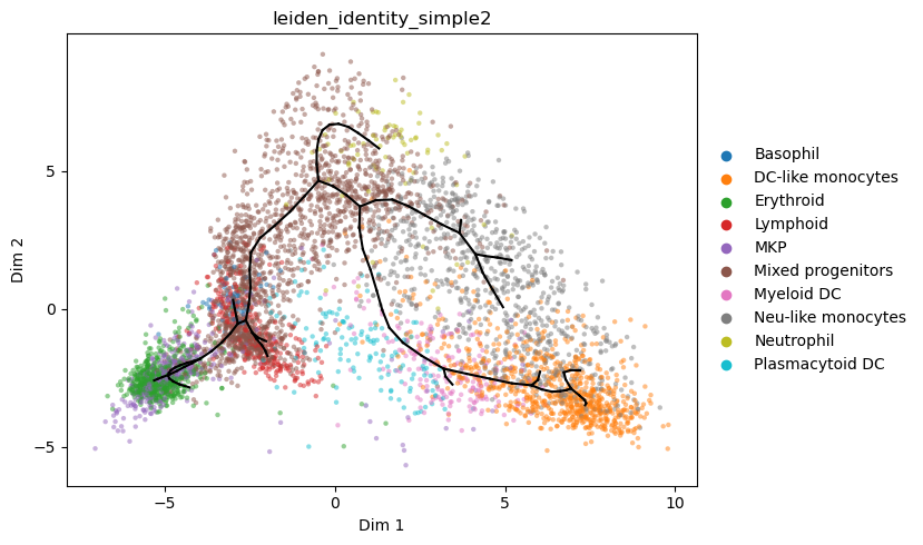
We can fine-tune the graph structure to: - add putative path from mixed progenitors to plasmacytoid DC - better fit paths for monocyte subtypes which are hard to capture - extend leaves of the graph to the very endpoints of the data distribution
[31]:
a_s2=a_s.copy()
st2.tl.del_path(a_s2,48,8)
st2.tl.add_path(a_s2,45,29)
st2.tl.add_path(a_s2,39,47,n_nodes=4)
st2.tl.add_path(a_s2,52,68)
st2.tl.del_path(a_s2,20,36)
st2.tl.del_path(a_s2,39,6)
st2.tl.del_path(a_s2,98,48)
st2.tl.del_path(a_s2,26,10)
st2.tl.del_path(a_s2,82,15)
st2.tl.add_path(a_s2,82,55)
st2.tl.refit_graph(a_s2,shift_nodes_pos={24 : a_s2.uns['epg']['node_pos'][24],# enforce same endpoint for monocytes
                                         26 : a_s2.uns['epg']['node_pos'][24],})
st2.tl.extend_leaves(a_s2,LeafIDs=np.array([18,12,98,45,48,24,50,32]),Mode="QuantDists",ControlPar=.7)
Performing simulated annealing. This may take a while
Performing simulated annealing. This may take a while
Performing simulated annealing. This may take a while
Performing simulated annealing. This may take a while
Performing simulated annealing. This may take a while
Performing simulated annealing. This may take a while
Performing simulated annealing. This may take a while
Performing simulated annealing. This may take a while
(8, 14)
(103, 14)
[32]:
st2.tl.project_graph(a_s2, to_basis='X_umap', key='epg')
st2.pl.graph(a_s2,color=['leiden_identity_simple2'],alpha=.5,size=10,fig_size=(16,10),show_text=1)
st2.pl.graph(a_s2,color=['leiden_identity_simple2'],alpha=.5,size=10,fig_size=(8,5),key='epg_from_X_dr_to_X_umap')
/home/jo/anaconda3/envs/stream2/lib/python3.8/site-packages/elpigraph/utils.py:403: RuntimeWarning: invalid value encountered in divide
  proj = (np.dot(X_embed.T, R) / R.sum(axis=0)).T
Now that we have the final graph we can compute pseudotime for further analyses
[33]:
adata_integrated.uns=a_s2.uns.copy()
st2.tl._elpigraph._store_graph_attributes(adata_integrated,adata_integrated.obsm['X_pca_transp_emd'],'epg')
st2.tl.infer_pseudotime(adata_integrated,40)
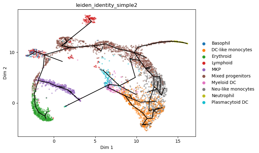
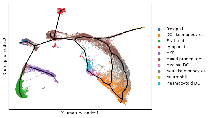
We can obtain a nicer 2D representation of nodes, e.g. by recomputing a UMAP directly including them
[34]:
# dummy anndata
a=sc.AnnData(np.concatenate((adata_integrated.obsm['X_pca_transp_emd'],adata_integrated.uns['epg']['node_pos'])))
sc.pp.neighbors(a,n_neighbors=50,metric='cosine')
sc.tl.umap(a,min_dist=0.05)

# store results
adata_integrated.obsm['X_umap_w_nodes']=a.obsm['X_umap'][:len(adata_integrated)]
adata_integrated.uns['umap_nodes']=a.obsm['X_umap'][len(adata_integrated):]

# plot
ax=plt.subplot()
_=sc.pl.embedding(adata_integrated,'X_umap_w_nodes',size=3,alpha=.5,
                  color='leiden_identity_simple2',show=False,return_fig=False,ax=ax)
ax.set_title(None)
ax.plot(adata_integrated.uns['umap_nodes'][adata_integrated.uns['epg']['edge'].T,0],
        adata_integrated.uns['umap_nodes'][adata_integrated.uns['epg']['edge'].T,1], c='k',linewidth=2)
plt.show()
/tmp/ipykernel_2000/3214916952.py:2: FutureWarning: X.dtype being converted to np.float32 from float64. In the next version of anndata (0.9) conversion will not be automatic. Pass dtype explicitly to avoid this warning. Pass `AnnData(X, dtype=X.dtype, ...)` to get the future behavour.
  a=sc.AnnData(np.concatenate((adata_integrated.obsm['X_pca_transp_emd'],adata_integrated.uns['epg']['node_pos'])))
/home/jo/anaconda3/envs/stream2/lib/python3.8/site-packages/scanpy/plotting/_tools/scatterplots.py:392: UserWarning: No data for colormapping provided via 'c'. Parameters 'cmap' will be ignored
  cax = scatter(
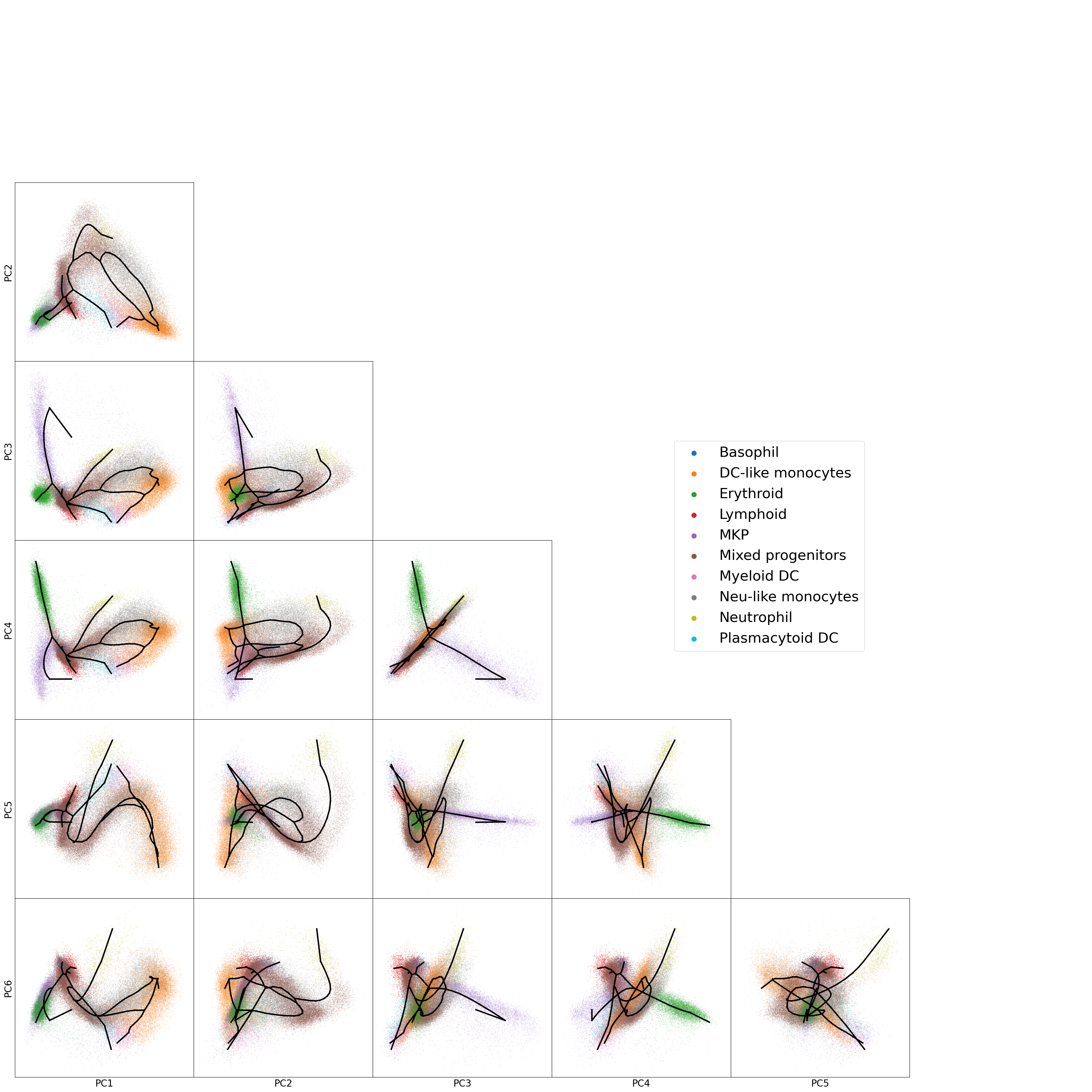
We can also plot various combination of PCs to get a better high-dimensional picture
[35]:
n_comps=6
f,axs=plt.subplots(n_comps,n_comps,figsize=(32,32),sharex='col',sharey='row')
for i in range(n_comps):
    for j in range(i+1,n_comps):

        _=sc.pl.embedding(adata_integrated,'X_pca_transp_emd',dimensions=(i,j),size=3,alpha=.5,
                        color='leiden_identity_simple2',show=False,return_fig=False,ax=axs[j,i])

        handles, labels = axs[j,i].get_legend_handles_labels()
        axs[j,i].get_legend().remove()
        axs[j,i].set_title(None)
        axs[j,i].plot(adata_integrated.uns['epg']['node_pos'][adata_integrated.uns['epg']['edge'].T,i],
                      adata_integrated.uns['epg']['node_pos'][adata_integrated.uns['epg']['edge'].T,j],
                      c='k',linewidth=3)

        if i==0:
            axs[j,i].set_ylabel(f'PC{j+1}',fontsize=20)
        else:
            axs[j,i].set_ylabel(None)
        if j==(n_comps-1):
            axs[j,i].set_xlabel(f'PC{i+1}',fontsize=20)
        else:
            axs[j,i].set_xlabel(None)

        if i<j:
            axs[i,i].axis('off')
            axs[i,j].axis('off')
axs[-1,-1].axis('off')
lgnd=f.legend(handles, labels, loc='center right',bbox_to_anchor=[.8, 0.5],prop={'size': 30})
for handle in lgnd.legendHandles:
    handle.set_sizes([100.0])
plt.tight_layout(pad=0,w_pad=0)
plt.show()
/tmp/ipykernel_2000/2761055043.py:30: MatplotlibDeprecationWarning: The legendHandles attribute was deprecated in Matplotlib 3.7 and will be removed two minor releases later. Use legend_handles instead.
  for handle in lgnd.legendHandles:
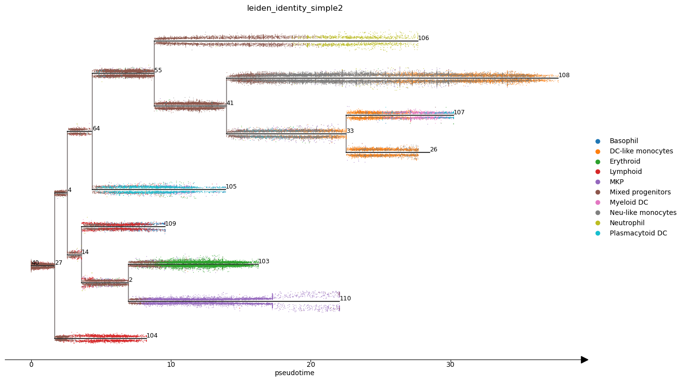
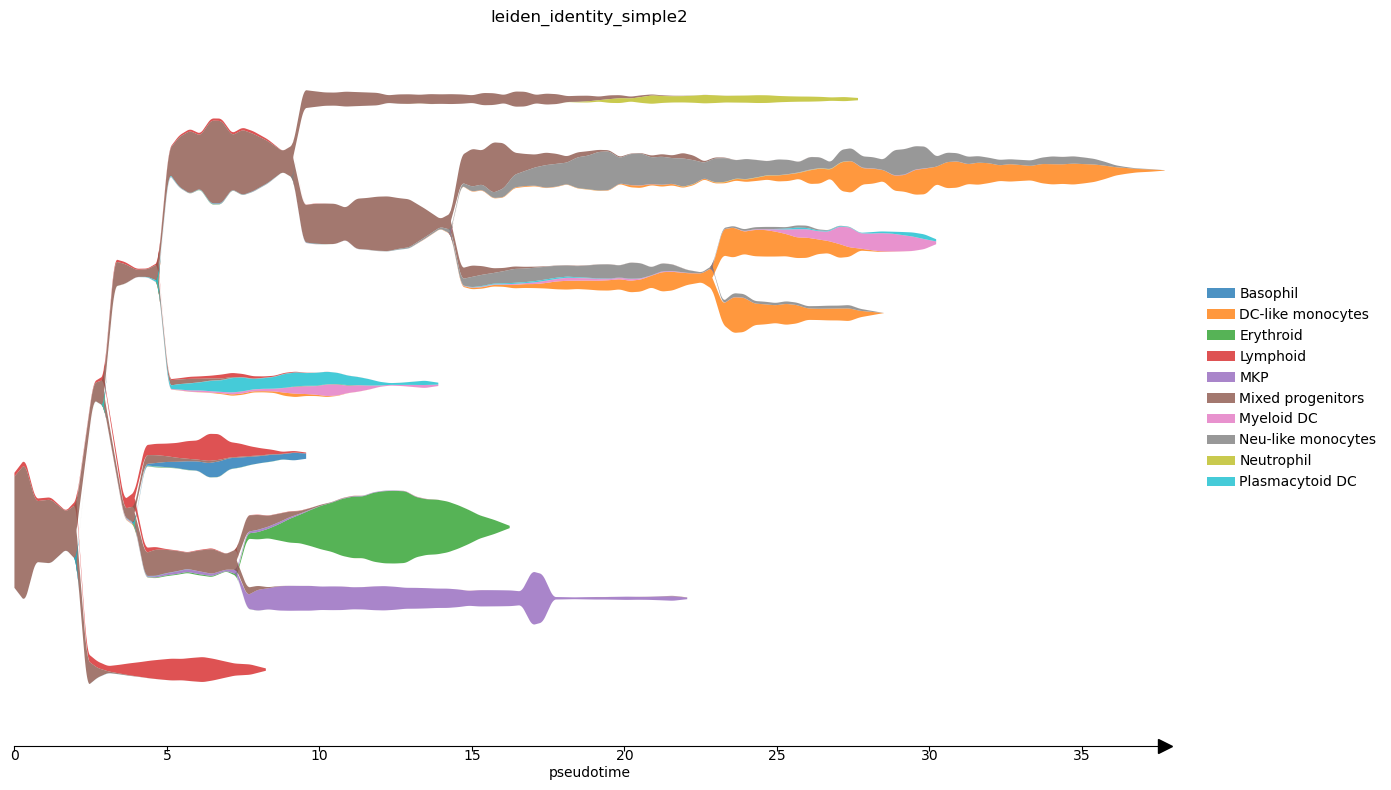
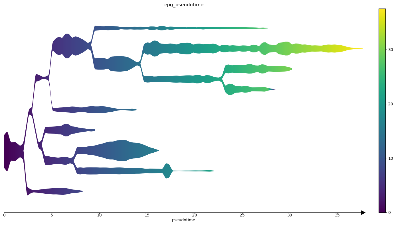
Finally we can produce STREAM plots.
[36]:
st2.pl.stream_sc(adata_integrated,40,dist_scale=.25,preference=[64],color=['leiden_identity_simple2'],fig_size=(14,8),size=1)
st2.pl.stream(adata_integrated,40,preference=[64],color=['leiden_identity_simple2'],fig_size=(14,8),dist_scale=2,factor_min_win=1.3,factor_num_win=4)
st2.pl.stream(adata_integrated,40,preference=[64],color=['epg_pseudotime'],fig_size=(14,8),dist_scale=2,factor_min_win=1.3,factor_num_win=4)
[ ]: